Բաց թողնել հիմնական բովանդակությունը

Ինչպե՞ս փոխել բանաձևը տեքստի տողի Excel- ում:

Սովորաբար Microsoft Excel- ը ցույց կտա հաշվարկված արդյունքները, երբ բանաձեւեր եք մուտքագրում բջիջներում: Այնուամենայնիվ, երբեմն կարող է անհրաժեշտ լինել բջիջում ցույց տալ միայն բանաձևը, ինչպիսիք են = ՀԱՇՎԱՊԱՀ ("000", "- 2"), ինչպե՞ս կվարվեք դրանով: Այս խնդիրը լուծելու մի քանի եղանակ կա.

Փոխակերպեք բանաձևը տեքստի տողի ՝ «Գտիր և փոխարինիր» հատկությամբ

Բանաձևը վերափոխեք տեքստի տողի ՝ օգտագործողի կողմից սահմանված գործառույթով

Փոխակերպեք բանաձևը տեքստի տողի կամ հակառակը ՝ միայն մեկ կտտոցով


Ենթադրելով, որ C սյունակում ունեք բանաձևերի շարք, և անհրաժեշտ է սյունը ցույց տալ բնօրինակ բանաձևերով, բայց ոչ դրանց հաշվարկված արդյունքներով, ինչպես ցույց են տրված հետևյալ նկարները.

doc-convert-formula-text-1-1 2 doc-convert-formula-text-2-2

Այս աշխատանքը լուծելու համար Գտնել եւ փոխարինել առանձնահատկությունը կարող է օգնել ձեզ, խնդրում ենք վարվել հետևյալ կերպ.

1. Ընտրեք հաշվարկված արդյունքի բջիջները, որոնք ցանկանում եք փոխարկել տեքստի տողի:

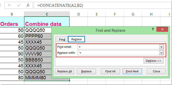
2. Այնուհետեւ սեղմեք Ctrl + H ստեղները միասին բացելու համար Գտնել եւ փոխարինել երկխոսության տուփ, երկխոսության մեջ, տակ Փոխարինել էջանիշ, մուտքագրեք հավասար = մուտք գործել Գտեք ինչ տեքստային տուփ և մուտքագրեք '= մեջ Փոխարինել տեքստային տուփ, տես նկարի նկարը.

doc-convert-formula-text-3-3

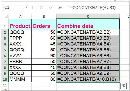
3. Այնուհետեւ կտտացրեք Փոխարինեք բոլորը կոճակը, դուք կարող եք տեսնել, որ բոլոր հաշվարկված արդյունքները փոխարինվում են բնօրինակ բանաձևի տեքստային տողերով, տես նկարի նկարը.

doc-convert-formula-text-4-4


Հետևյալ VBA կոդը նույնպես կարող է օգնել ձեզ հեշտությամբ լուծվել դրա հետ:

1, Պահեք պահեք ալտ + F11 Excel- ի ստեղները, և այն բացում է Microsoft Visual Basic հավելվածների համար պատուհան.

2: Սեղմեք Տեղադրել > Մոդուլներ, և տեղադրեք հետևյալ մակրոը ՝ Մոդուլի պատուհան.

Function ShowF(Rng As Range)
ShowF = Rng.Formula
End Function

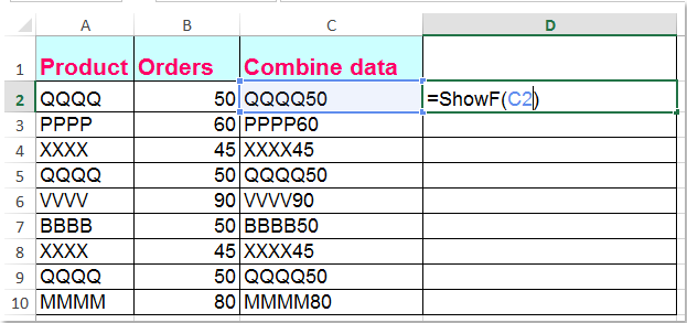
3, Դատարկ խցում, ինչպիսին է բջիջը D2, մուտքագրեք բանաձև = ShowF (C2).

doc-convert-formula-text-5-5

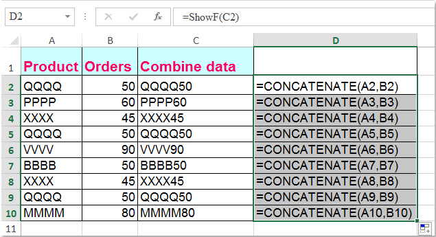
4. Դրանից հետո կտտացրեք Բջջային D2- ին և քաշեք Լրացնելու բռնակը ձեզ համար անհրաժեշտ միջակայքում:

doc-convert-formula-text-6-6


Եթե ​​դուք ունեք Excel- ի համար նախատեսված գործիքներԻր Ձևակերպումը տեքստի վերածել գործառույթը, դուք կարող եք փոխել բազմաթիվ բանաձևեր տեքստային տողերի միայն մեկ հպումով:

Excel- ի համար նախատեսված գործիքներ : ավելի քան 300 հարմար Excel հավելվածներով, 30 օրվա ընթացքում առանց սահմանափակումների փորձեք անվճար. 

Տեղադրելուց հետո Excel- ի համար նախատեսված գործիքներԽնդրում եմ արեք հետևյալ կերպ

1, Ընտրեք բանաձևերը, որոնք ցանկանում եք փոխարկել:

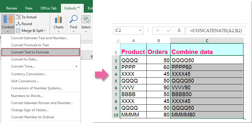
2: Սեղմեք Կուտոլս > Պարունակություն > Ձևակերպումը տեքստի վերածել, և ձեր ընտրած բանաձևերը միանգամից փոխակերպվել են տեքստի տողերի, տե՛ս նկարը.

Խորհուրդներ. Եթե ցանկանում եք բանաձևի տեքստի տողերը վերափոխել հաշվարկված արդյունքների, խնդրում ենք պարզապես կիրառել Փոխարկել տեքստը բանաձևի օգտակարությանը, ինչպես ցույց է տրված հետևյալ նկարը.

Եթե ​​ցանկանում եք ավելին իմանալ այս հատկության մասին, այցելեք Ձևակերպումը տեքստի վերածել.

Ներբեռնեք և անվճար փորձեք Kutools- ը Excel- ի համար:


Excel- ի համար նախատեսված գործիքներ. Excel- ի ավելի քան 300 հարմարավետ հավելումներով, 30 օրվա ընթացքում անվճար փորձեք առանց սահմանափակումների: Ներբեռնեք և անվճար փորձեք հիմա:

Գրասենյակի արտադրողականության լավագույն գործիքները

🤖 Kutools AI օգնականՀեղափոխություն կատարել տվյալների վերլուծության հիման վրա՝ Խելացի կատարում   |  Ստեղծեք ծածկագիր  |  Ստեղծեք հատուկ բանաձևեր  |  Վերլուծել տվյալները և ստեղծել գծապատկերներ  |  Invoke Kutools-ի գործառույթները...
Հանրաճանաչ հատկություններ: Գտեք, ընդգծեք կամ նույնականացրեք կրկնօրինակները   |  Deleteնջել դատարկ շարքերը   |  Միավորել սյունակները կամ բջիջները՝ առանց տվյալների կորստի   |   Կլոր առանց բանաձևի ...
Super Փնտրել: Բազմաթիվ չափանիշների VLookup    Բազմակի արժեք VLookup  |   VLookup բազմաթիվ թերթերում   |   Fuzzy Փնտրել ....
Ընդլայնված բացվող ցուցակ: Արագ ստեղծեք բացվող ցուցակը   |  Կախված բացվող ցուցակ   |  Բազմակի ընտրություն Drop Down ցուցակ ....
Սյունակի կառավարիչ: Ավելացրեք որոշակի քանակությամբ սյունակներ  |  Տեղափոխել սյունակները  |  Փոխարկել թաքնված սյունակների տեսանելիության կարգավիճակը  |  Համեմատեք միջակայքերը և սյունակները ...
Առանձնահատկություններ: Ցանցի կենտրոնացում   |  Դիզայնի տեսք   |   Մեծ Formula Bar    Աշխատանքային գրքույկի և թերթիկների կառավարիչ   |  Ռեսուրսների գրադարան (Ավտոմատ տեքստ)   |  Ամսաթիվ ընտրող   |  Միավորել աշխատանքային թերթերը   |  Գաղտնագրել/գաղտնազերծել բջիջները    Ուղարկեք նամակներ ըստ ցանկի   |  Սուպեր զտիչ   |   Հատուկ զտիչ (զտել թավ/շեղ/շեղված...) ...
Լավագույն 15 գործիքների հավաքածու12 Տեքստ Գործիքներ (Ավելացրեք տեքստ, Հեռացնել նիշերը, ...)   |   50+ Աղյուսակ Տեսակներ (Գանտի աղյուսակը, ...)   |   40+ Գործնական Բանաձեւեր (Հաշվարկել տարիքը ՝ ելնելով ծննդյան տարեդարձից, ...)   |   19 միացում Գործիքներ (Տեղադրեք QR կոդ, Տեղադրեք նկար ուղուց, ...)   |   12 Փոխարկում Գործիքներ (Բառեր համարներ, Արտարժույթի փոխակերպումը, ...)   |   7 Միաձուլում և պառակտում Գործիքներ (Ընդլայնված կոմբինատ տողեր, Պառակտված բջիջներ, ...)   |   ... եւ ավելին

Լրացրեք ձեր Excel-ի հմտությունները Kutools-ի հետ Excel-ի համար և փորձեք արդյունավետությունը, ինչպես երբեք: Kutools-ը Excel-ի համար առաջարկում է ավելի քան 300 առաջադեմ առանձնահատկություններ՝ արտադրողականությունը բարձրացնելու և ժամանակ խնայելու համար:  Սեղմեք այստեղ՝ Ձեզ ամենաշատ անհրաժեշտ հատկանիշը ստանալու համար...

Նկարագրություն


Office Tab- ը Tabbed ինտերֆեյսը բերում է Office, և ձեր աշխատանքը շատ ավելի դյուրին դարձրեք

  • Միացնել ներդիրներով խմբագրումը և ընթերցումը Word, Excel, PowerPoint- ով, Հրատարակիչ, Access, Visio և Project:
  • Բացեք և ստեղծեք բազմաթիվ փաստաթղթեր նույն պատուհանի նոր ներդիրներում, այլ ոչ թե նոր պատուհաններում:
  • Բարձրացնում է ձեր արտադրողականությունը 50%-ով և նվազեցնում մկնիկի հարյուրավոր սեղմումները ձեզ համար ամեն օր:
Comments (20)
No ratings yet. Be the first to rate!
This comment was minimized by the moderator on the site
How do I convert the non matched value retrieved from vlookup into text??
This comment was minimized by the moderator on the site
The find and replace facility is extremely useful, I didn't expect it to work when showing formulae instead of result. Thanks
This comment was minimized by the moderator on the site
[quote name="Jennifer"]Hi, is there a short cut method to concatenate 230 cells in excel to and text string, or do I have to add each cell to the concatenate formula with at divider? Thanks so much! Converting the range of data into Table (Insert>Table) may help you. As and when a row of data is appended to and inserted in to an existing table, formulas and format of number in columns are applied to the new data also. File size may increase in Table mode. The Table may be changed to Range mode later (Table tools>Tools>convert to range to reduce file size if needed. Maintaining data in Table mode has advantages.
This comment was minimized by the moderator on the site
The Visual Basic editor option didn't work for me - kept returning errors about it needing to be the first row?
This comment was minimized by the moderator on the site
Hi, is there a short cut method to concatenate 230 cells in excel to and text string, or do I have to add each cell to the concatenate formula with at divider? Thanks so much!
This comment was minimized by the moderator on the site
Inserting the “concatenation operator” (& or &” “&) among 230 Excel cells can be done in MS Word. This method is good enough if the task is not repetitive and if a Procedure is not available. (1) Arrange all the 230 cell-references (the text of which is to be merged in to one cell) in single column or single row in a Table in the merging order (use Excel worksheet and paste in Word). (2) Select the table and merge cells (Table Tools > Layout > Merge Cells) to get multi-line single-column Table with paragraph mark at the end of each line except last line. (3) Replaces all paragraph marks with commas (Editing > Replace; Find what = ^p and Replace with = ,). (4) Convert table to text to get content of each cell separated by a comma in a single paragraph. (5) Replaces all commas with concatenation-operator or operators, & or &” “& as required (Editing > Replace; Find what = , and Replace with = & or &” “&). (6) Prefix “=” to the paragraph. Required formula is ready in text form. Copy and paste in Excel; it becomes a formula. (7) The same result can be achieved in MS Excel also through Editing > Fill > Justify but with limitations. (a) Width of merged text that can be displayed is equal to the width of cell where Justify is applied. Superfluous text is written in cells below as separate text. (b) Numbers are to be converted to text (Formulas > Text > TEXT(Value, Format_text). I am an Excel user only and I am sorry for my earlier inappropriate suggestion.
This comment was minimized by the moderator on the site
i need to change my text which in column 115 gm to 115. how it is possible. need to change text in to value like 115 in next column.
This comment was minimized by the moderator on the site
Hi, if you use the text to column feature you can do this. highlight the column in question, click on text to column, step through the process. It will ask you what your delimiter is, if there is a space between the quantity and the measurement (115 gm) you can use the space as your delimiter. PS... add a column to the right of your data column just incase it does something wonky on you.
This comment was minimized by the moderator on the site
I need to convert text from value to sort a large data. please help. For Example 115 gm (this is in shown as text) I need only 115 in next column to sort. Please reply help in this regards
This comment was minimized by the moderator on the site
[quote]I need to convert text from value to sort a large data. please help. For Example 115 gm (this is in shown as text) I need only 115 in next column to sort. Please reply help in this regardsBy Ahmed[/quote] 897/5000 Hi, if the numbers inside the text string are in correlative form, try this, in the formula bar type B1 (if the data column is in A1): = MID (A1, MIN (IFERROR (FIND ({0; 1; 2; 3; 4; 5; 6; 7; 8; 9}, A1), "")), COUNT (1: $ 98), 1))) And then press Ctrl + Shift + Enter because it is a matrix formula, ie at the beginning and end of the formula will appear {y}. Note that I use the comma (,), but it is likely that you must use the semicolon (;) to create both the array of digits and to separate the arguments of the function. I apologize if there is something wrong with the translation from Spanish, if it gives you an error in case I copy the formula in that language: = EXTRACT (A1, MIN (IF YOU FIND ({0; 1; 2; 3; 4; 5; 6; 7; 8; 9}, A1) , FILA ($ 1: $ 98), 1))) Original by Moisés Ortíz (https://exceltotal.com/extraer-numeros-de-una-celda-en-excel/)
This comment was minimized by the moderator on the site
I need to copy the results from a column with a formula to another column but I want just the results copied not the formula. In other words, I have a column with addresses. I have created another column and using a formula I have removed the house number and now just see the street name. Now I need to copy those results (street names only) to another column in a different spreadsheet, but when I try to do this it only copies the formula which of course then gives me the #ref error because the starting data isn't available. Any suggestions?
This comment was minimized by the moderator on the site
I am here because I have been trying to resolve a problem with file names. I have some 40 files with identical names except for the year 2 digits. I simply need to construct the file name (eg C:Docs\Research\...\[Year72.xlsx]Test!$B$10 ro retrieve the data out of that particular file cell B10. I can build the file name in the working workbook,and create the address (using Address), but cannot extract the data in that file cell using Indirect, as Indirect does not access closed files, and opening so many files is not an option. Have we got Microsoft or is there a workaround? as this requirement must be common. :
This comment was minimized by the moderator on the site
Assuming your text function is in A1; 1. Create a text string elsewhere which includes the equals sign eg. =CONCATENATE("@=",A1) 2. This will give you @=10+20, which you can now copy (paste values) to wherever you want it. 3. Finally, simply replace the @= with = using Ctrl+H as above. It's three steps, but it avoids VBA and doesn't take long.
There are no comments posted here yet
Load More
Please leave your comments in English
Posting as Guest
×
Rate this post:
0   Characters
Suggested Locations