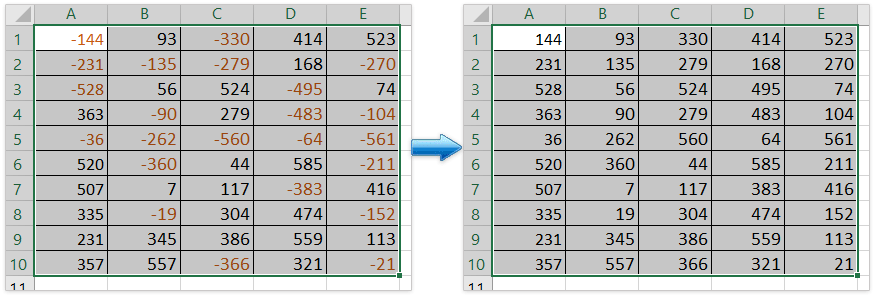
Բացասական թվերը դրական թվերի կարող եք փոխել հետևյալ քայլերով.

1, Մուտքագրեք համարը -1 դատարկ վանդակում, ապա ընտրեք այս բջիջը և սեղմեք Ctrl + C կրկնօրինակները:

2, Ընտրեք տիրույթի բոլոր բացասական թվերը, սեղմեք աջով և ընտրեք Տեղադրել հատուկ ... համատեքստային ընտրացանկից: Տեսեք,

Նշումներ:
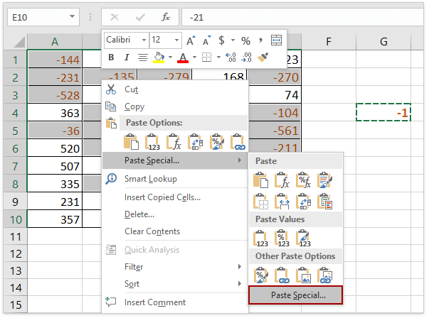
(1) հոլդինգ Ctrl ստեղնը, դուք կարող եք ընտրել բոլոր բացասական թվերը մեկ առ մեկ կտտացնելով դրանք;
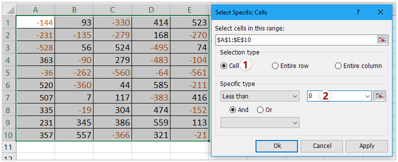
(2) Եթե Excel- ի համար տեղադրել եք Kutools, կարող եք կիրառել այն Ընտրեք հատուկ բջիջներ հատկություն ՝ բոլոր բացասական թվերն արագ ընտրելու համար: Անցկացրեք անվճար փորձություն:

3, Եվ ա Տեղադրել հատուկ կցուցադրվի երկխոսության տուփը, ընտրեք բոլորը տարբերակ ՝ սկսած մածուկընտրեք Բաղադրյալ տարբերակ ՝ սկսած ԳործողությունՀամար OK, Տեսեք,

4, Բոլոր ընտրված բացասական թվերը կվերածվեն դրական թվերի: Numberնջեք -1 թիվը, որքան անհրաժեշտ է: Տեսեք,

Excel- ում նշված տիրույթում հեշտությամբ փոխեք բացասական թվերը դրականի

Համեմատելով բացասական նշանը բջիջներից մեկ առ մեկ ձեռքով հեռացնելու հետ, Kutools Excel- ի համար Փոխել արժեքների նշանը առանձնահատկությունն ապահովում է չափազանց հեշտ միջոց `բոլոր բացասական թվերը ընտրության մեջ դրականի արագ փոխելու համար:

Որպես Excel մասնագետ, նաև կարող եք գործարկել VBA կոդը ՝ բացասական թվերը դրական թվերի փոխելու համար:

1, Սեղմեք Alt + F11 ստեղները ՝ Microsoft Visual Basic հավելվածների համար պատուհանը բացելու համար:

2, Windowուցադրված կլինի նոր պատուհան: Սեղմել Տեղադրել > Մոդուլներ, ապա մուտքագրեք հետևյալ կոդերը մոդուլում.

Sub Positive
Dim Cel As Range
For Each Cel In Selection
If IsNumeric(Cel.Value) Then
Cel.Value = Abs(Cel.Value)
End If
Next Cel
End Sub

3. Այնուհետեւ կտտացրեք Վազում կոճակը կամ սեղմել F5 դիմումը գործարկելու բանալին, և բոլոր բացասական թվերը կփոխվեն դրական թվերի: Տեսեք,

Excel- ի օգտվողների մեծ մասը չի ցանկանում օգտագործել VBA կոդ, կա՞ն արդյոք արագ հնարքներ բացասական թվերը դրականի վերափոխելու համար: Kutools համար Excel կարող է օգնել ձեզ հեշտությամբ և հարմարավետորեն հասնել դրան:

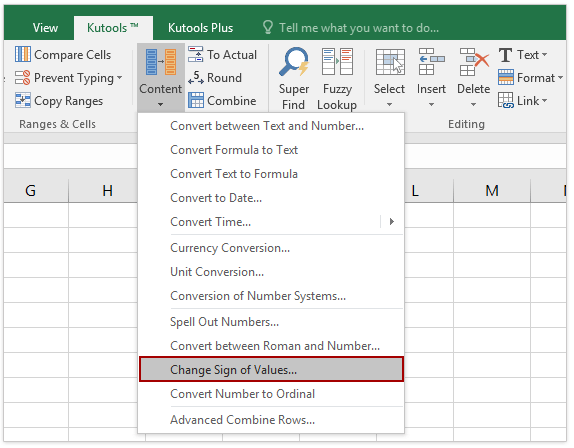
1, Ընտրեք ընդգրկույթ, ներառյալ բացասական թվերը, որոնք ցանկանում եք փոխել, և կտտացրեք Կուտոլս > Պարունակություն > Փոխել արժեքների նշանը.

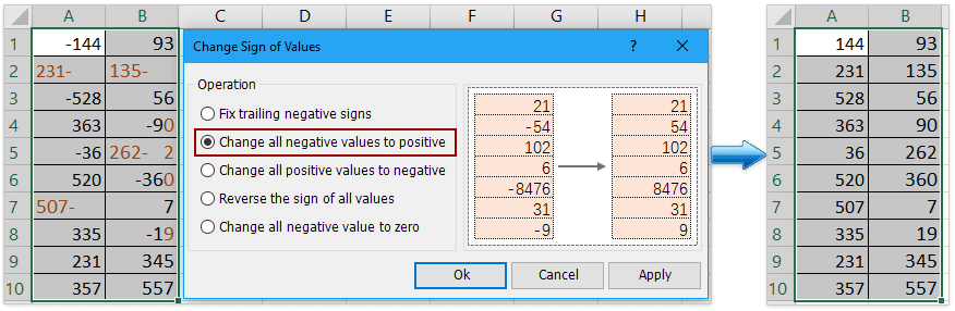
2, Check Բոլոր բացասական արժեքները փոխեք դրականի տակ Գործողությունեւ սեղմեք Ok, Տեսեք,

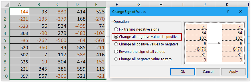
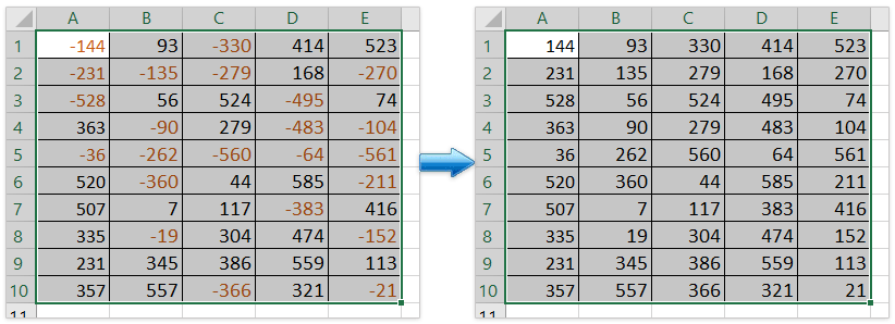
Այժմ կտեսնեք, որ բոլոր բացասական թվերը վերածվում են դրական թվերի, ինչպես ցույց է տրված ստորև:

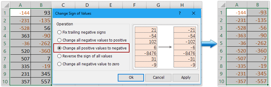
Նշում: Սրանով Արժեքների նշանի փոփոխություն հատկությունը, դուք նաև կարող եք ուղղել հետևող բացասական նշանները, բոլոր դրական թվերը փոխել բացասականների, բոլոր արժեքների նշանը հակադարձել և բոլոր բացասական արժեքները դարձնել զրո: Անցկացրեք անվճար փորձություն:

(1) Նշված տիրույթում արագ փոխեք բոլոր դրական արժեքները բացասականների ՝

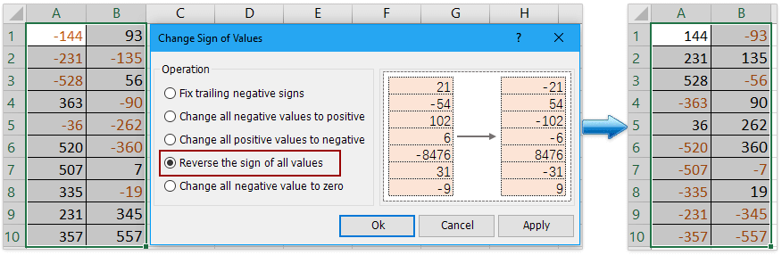
(2) Նշված տիրույթում հեշտությամբ հետ շրջեք բոլոր արժեքների նշանը.

(3) Նշված տիրույթում բոլոր բացասական արժեքները հեշտությամբ փոխեք զրոյի.

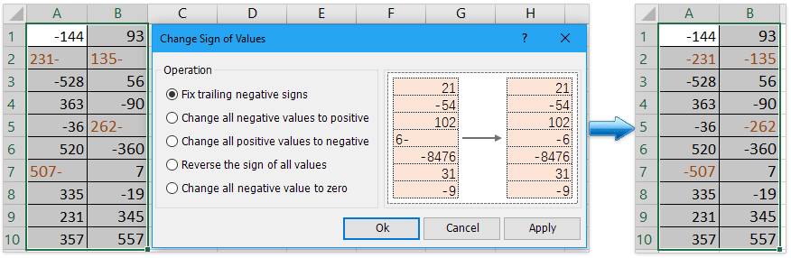
(4) Հեշտությամբ շտկեք հետևյալ բացասական նշանները նշված տիրույթում.

Դրական թվերը փոխեք բացականի

Բջիջներում արժեքների հակառակ նշաններ

Ուղղեք բջիջներում հետապնդող բացասական նշանները

Բացասական թիվը փոխել զրոյի