Բաց թողնել հիմնական բովանդակությունը

Ինչպե՞ս Excel- ում տող դուրս բերել երկու տարբեր նիշերի միջև:

Եթե ​​ունեք Excel- ի տողի ցուցակ, որը ձեզ հարկավոր է դուրս բերել տողի մի մասը երկու նիշի միջև, ինչպես ցույց է տրված ստորև նշված էկրանի նկարը, ինչպե՞ս կարգավորել այն հնարավորինս արագ: Այստեղ ես ներկայացնում եմ որոշ մեթոդներ այս աշխատանքը լուծելու վերաբերյալ:

Բանաձևերով արդյունահանեք մասի տողը երկու տարբեր նիշերի միջև

Բանաձևերով դուրս բերեք մասի տողը երկու նույն նիշերի միջև

Excel- ի համար Kutools- ով հանեք մասի տողը երկու նիշի միջևլավ գաղափար 3


Բանաձևերով արդյունահանեք մասի տողը երկու տարբեր նիշերի միջև

Երկու տարբեր նիշերի միջև մասի տողը հանելու համար կարող եք անել հետևյալ կերպ.

Ընտրեք բջիջ, որը կտեղադրեք արդյունքը, մուտքագրեք այս բանաձևը =MID(LEFT(A1,FIND(">",A1)-1),FIND("<",A1)+1,LEN(A1))եւ սեղմեք Enter բանալի.
doc քաղվածք տողը երկու նիշի միջև 1

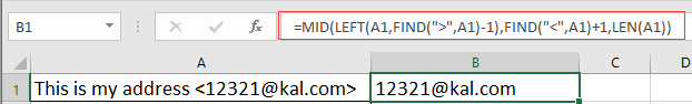
ՆշումA1- ը տեքստային բջիջ է, > և < այն երկու նիշն են, որոնց միջեւ ցանկանում եք տող դուրս բերել:


Բանաձևերով դուրս բերեք մասի տողը երկու նույն նիշերի միջև

Եթե ​​ցանկանում եք մասի տողը դուրս բերել երկու նույն նիշերի միջև, ապա կարող եք անել հետևյալը.

Ընտրեք բջիջ, որը կտեղադրեք արդյունքը, մուտքագրեք այս բանաձևը =SUBSTITUTE(MID(SUBSTITUTE("/" & A3&REPT(" ",6),"/",REPT(",",255)),2*255,255),",","")եւ սեղմեք Enter բանալի.
doc քաղվածք տողը երկու նիշի միջև 2

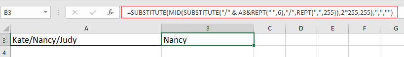
Նշում: A3- ը տեքստի բջիջ է, / այն կերպարն է, որի միջեւ ցանկանում եք արդյունահանել:

Excel- ի համար Kutools- ով հանեք մասի տողը երկու նիշի միջև

Եթե ​​դուք ունեք Kutools for Excel, Դուք նաև կարող եք հատված տող դուրս բերել երկու տեքստի միջև:

Excel- ի համար նախատեսված գործիքներ, ավելի քան 300 հարմար գործառույթներ, ավելի հեշտացնում է ձեր գործերը: 

Տեղադրելուց հետո Excel- ի համար նախատեսված գործիքներ, խնդրում ենք վարվել ինչպես ստորև ՝(Անվճար ներբեռնեք Kutools- ի համար Excel- ը հիմա!)

1. Ընտրեք բջիջ, որը կտեղադրի արդյունահանվող տողը, ապա կտտացրեք Կուտոլս > Ֆորմուլա > Բանաձևի օգնական.
doc քաղվածք տողը երկու նիշի միջև 3

2. Մեջ Բանաձևի օգնական երկխոսություն, .ստուգում ֆիլտր վանդակը, ապա մուտքագրեք «նախկին» տեքստային տուփի մեջ, արդյունահանման վերաբերյալ բոլոր բանաձևերը կցուցադրվեն Ընտրեք բանաձեւ Բաժին ընտրել Տողեր հանիր նշված տեքստի միջև, ապա գնացեք աջ Փաստարկների մուտքագրում բաժնում ընտրեք այն բջիջը, որի մեջ ցանկանում եք ենթաշարք դուրս բերել Բջիջ, ապա մուտքագրեք երկու տեքստերը, որոնց միջեւ ցանկանում եք արդյունահանել:
doc kutools- ը տող է հանում երկու տեքստի միջեւ 2

3: սեղմեք Ok, ապա արդյունահանվել է ձեր նշած երկու տեքստերի ենթատողը, քաշեք ներքև լրացնելու բռնակը ներքևի յուրաքանչյուր բջիջներից ենթագլուխ հանելու համար:
doc kutools- ը տող է հանում երկու տեքստի միջեւ 3

doc kutools- ը տող է հանում երկու տեքստի միջեւ 4

Գրասենյակի արտադրողականության լավագույն գործիքները

🤖 Kutools AI օգնականՀեղափոխություն կատարել տվյալների վերլուծության հիման վրա՝ Խելացի կատարում   |  Ստեղծեք ծածկագիր  |  Ստեղծեք հատուկ բանաձևեր  |  Վերլուծել տվյալները և ստեղծել գծապատկերներ  |  Invoke Kutools-ի գործառույթները...
Հանրաճանաչ հատկություններ: Գտեք, ընդգծեք կամ նույնականացրեք կրկնօրինակները   |  Deleteնջել դատարկ շարքերը   |  Միավորել սյունակները կամ բջիջները՝ առանց տվյալների կորստի   |   Կլոր առանց բանաձևի ...
Super Փնտրել: Բազմաթիվ չափանիշների VLookup    Բազմակի արժեք VLookup  |   VLookup բազմաթիվ թերթերում   |   Fuzzy Փնտրել ....
Ընդլայնված բացվող ցուցակ: Արագ ստեղծեք բացվող ցուցակը   |  Կախված բացվող ցուցակ   |  Բազմակի ընտրություն Drop Down ցուցակ ....
Սյունակի կառավարիչ: Ավելացրեք որոշակի քանակությամբ սյունակներ  |  Տեղափոխել սյունակները  |  Փոխարկել թաքնված սյունակների տեսանելիության կարգավիճակը  |  Համեմատեք միջակայքերը և սյունակները ...
Առանձնահատկություններ: Ցանցի կենտրոնացում   |  Դիզայնի տեսք   |   Մեծ Formula Bar    Աշխատանքային գրքույկի և թերթիկների կառավարիչ   |  Ռեսուրսների գրադարան (Ավտոմատ տեքստ)   |  Ամսաթիվ ընտրող   |  Միավորել աշխատանքային թերթերը   |  Գաղտնագրել/գաղտնազերծել բջիջները    Ուղարկեք նամակներ ըստ ցանկի   |  Սուպեր զտիչ   |   Հատուկ զտիչ (զտել թավ/շեղ/շեղված...) ...
Լավագույն 15 գործիքների հավաքածու12 Տեքստ Գործիքներ (Ավելացրեք տեքստ, Հեռացնել նիշերը, ...)   |   50+ Աղյուսակ Տեսակներ (Գանտի աղյուսակը, ...)   |   40+ Գործնական Բանաձեւեր (Հաշվարկել տարիքը ՝ ելնելով ծննդյան տարեդարձից, ...)   |   19 միացում Գործիքներ (Տեղադրեք QR կոդ, Տեղադրեք նկար ուղուց, ...)   |   12 Փոխարկում Գործիքներ (Բառեր համարներ, Արտարժույթի փոխակերպումը, ...)   |   7 Միաձուլում և պառակտում Գործիքներ (Ընդլայնված կոմբինատ տողեր, Պառակտված բջիջներ, ...)   |   ... եւ ավելին

Լրացրեք ձեր Excel-ի հմտությունները Kutools-ի հետ Excel-ի համար և փորձեք արդյունավետությունը, ինչպես երբեք: Kutools-ը Excel-ի համար առաջարկում է ավելի քան 300 առաջադեմ առանձնահատկություններ՝ արտադրողականությունը բարձրացնելու և ժամանակ խնայելու համար:  Սեղմեք այստեղ՝ Ձեզ ամենաշատ անհրաժեշտ հատկանիշը ստանալու համար...

Նկարագրություն


Office Tab- ը Tabbed ինտերֆեյսը բերում է Office, և ձեր աշխատանքը շատ ավելի դյուրին դարձրեք

  • Միացնել ներդիրներով խմբագրումը և ընթերցումը Word, Excel, PowerPoint- ով, Հրատարակիչ, Access, Visio և Project:
  • Բացեք և ստեղծեք բազմաթիվ փաստաթղթեր նույն պատուհանի նոր ներդիրներում, այլ ոչ թե նոր պատուհաններում:
  • Բարձրացնում է ձեր արտադրողականությունը 50%-ով և նվազեցնում մկնիկի հարյուրավոր սեղմումները ձեզ համար ամեն օր:
Comments (35)
No ratings yet. Be the first to rate!
This comment was minimized by the moderator on the site
Bonjour,

je souhaite extraire de ce texte (USD) 934.915765 (30-11-2022) le numero 934.915765, ce que je souhaite c'est faire un extrait de tout ce qui est entre (USD) et (30-11-2022)
This comment was minimized by the moderator on the site
Hi, please try this formula:
=LEFT((MID(I1,FIND(" ",I1)+1,256)),FIND(" ",(MID(I1,FIND(" ",I1)+1,256)),1)-1)
I1 is the cell that you want to extract number.
This comment was minimized by the moderator on the site
Hi, try this formula please:
=IFERROR(MID(A1,FIND("CG",A1),11),IFERROR(MID(A1,FIND("CP",A1),11),IFERROR(MID(A1,FIND("CV",A1),11),IFERROR(MID(A1,FIND("CD",A1),11),IFERROR(MID(A1,FIND("CC",A1),11),MID(A1,FIND("CO",A1),11))))))

If there is no match string, it returns #VALUE! error.
This comment was minimized by the moderator on the site
Hello, can you please help me with extracting a code from a cell? The code is always 11 characters long and it can start with either CC, CP, CV, CO, CG or CD. If it helps, it also ends with a number always. The code does not have a fixed position, it can be in the beginning, middle or end.
I tried this formula =MID(A2,FIND("CP",A2),11) but, as you see, it only finds the ones starting with CP.

An example of what the cell might contain is:
Text text CG1234dh201 text 123 text

Thank you!
This comment was minimized by the moderator on the site
Hi, I have an issue which i am struggling to solve. So I have a number of answers and i want to separate into separate cells.

i.e. A: XYZ|B*: SDR|C: AQS|

I can separate but my issue is there loads of line with the asterisk moving to the correct answer for each question. How do i get my head around this?

I am currently using the below formula

=MID(A5,SEARCH("A:",cell ref)+2,SEARCH("|",A5)-SEARCH(":",cell ref)-1)
This comment was minimized by the moderator on the site
Hi, Mohannmed Faisal, from my understanding, your question is to extract XYZ, SDR and AQS separately into three cells. If so, please use formulas below separately:
=MID(A7,SEARCH("A:",A7)+3,3)
=MID(A7,SEARCH("B*:",A7)+4,3)
=MID(A7,SEARCH("|C:",A7)+4,3)
A7 is the cell that you use to extract.
Hope it help you.
This comment was minimized by the moderator on the site
Bonjour,

J'ai un texte AAMMJJ que je souhaite transformer en JJMMAAAA
This comment was minimized by the moderator on the site
Hi, GG, try this formula =TEXTE(date; "jj/mm/aaaa")
This comment was minimized by the moderator on the site
Hi How to get specific value from description like
Desc: Date: 2022-07-22 23:59:51 Node: VA10TWPSQL026 Type: TSM SM_SERVER_EVENT 2579 Resource: 1700 Message Key: TSM_VA10TWPSQL026

I want to get node value as VA10TWPSQL026
This comment was minimized by the moderator on the site
Hi, Sandhya, if the node value always has a fixed length (14-chars), you can try this formula: =MID(A1,SEARCH("Node",A1)+5,14) hope it do a favor for you.
This comment was minimized by the moderator on the site
Hola,

Me encantan tus foros.

Me podrias ayudar con esto?

Tengo una serie de columnas asi:

U CALIPER R/H/R 1J0615424H Es
N DOOR WINDOW SWITCH R/H/F 8E0959851D5PR Ebbett Audi
N TAILIGHT L/H - LENS & BODY - ON QTR - W/XENON H/LAMP 63217217311 Coombes Johnson European Ltd
U*GUARD R/H/F - REPLACE RET NUT ALSO 5G0821106A (V) Private Purchase

Lo que necesito extraer es el numero de parte de cada celda pero siempre esta en una posicion diferente, por ejemplo de la primer celda necesito solo 1J0615424H, de la segunda necesito extraer 8E0959851D5PR, de la tercera 63217217311 y de la ultima 5G0821106A

Muchas gracias

Anderson
This comment was minimized by the moderator on the site
Hallo,

Ik moet een stuk tekst extraheren uit een cel, maar kom er niet aan uit.

51420647 Ondersteuner Kringdirectie (Unfilled)
P_00040501 Productmanager Wendbare Pool Bedrijven (Unfilled)

De tekst die ik nodig heb ik is het middelste deel tussen de cijfers en (unfilled).
Welke formuler kan ik hiervoor gebruiken?
This comment was minimized by the moderator on the site
HelloI have an issue where I am trying to extract a number from a set of text and numbers in excel. This is an excerpt from the data I have:AUS23-7W
GER490-8W
MEX114-2M
MEX444-5M
MEX331-3W
US118-15W
ARG572-16W
Japan122-6W
Japan526-13W
ARG585-7W
Japan398-16W
Japan320-15W
ARG141-3Mo
Canada329-5W
US421-17Mo
Canada427-14W
I need to be able to extract just the number to the right of the dash. For example, I need Japan320-15W to return just the 15 in its own column. Is there a formula you could provide me with that can accomplish this? Many thanks!

This comment was minimized by the moderator on the site
Hello, Duggled, to solve your job, just need two steps. Firstly, select the text strings, and apply Text to Columns under Data tab, choose Delimited > Other, and type - into the textbox beside Other option, click Finish. In this step, your data has been split into two columns by deliliter -. Secondly, use the formula  =SUMPRODUCT(MID(0&B1, LARGE(INDEX(ISNUMBER(--MID(B1, ROW(INDIRECT("1:"&LEN(B1))), 1)) * ROW(INDIRECT("1:"&LEN(B1))), 0), ROW(INDIRECT("1:"&LEN(B1))))+1, 1) * 10^ROW(INDIRECT("1:"&LEN(B1)))/10)(A1 is the cell that you want to extract the number from, here you change it to your second column cell)then the numbers after - have been extracted. Or in the second step, you can apply VBA, or our handy tool, for more details, please visit:https://www.extendoffice.com/documents/excel/1622-excel-extract-number-from-string.html
This comment was minimized by the moderator on the site
This formula works well for pretty much everything except these data :MEX114-2M
MEX444-5M
MEX373-15M
MEX540-8M
MEX396-11M
MEX386-10M
MEX369-14M
MEX446-3M
MEX75-12M
MEX372-3M
MEX178-6M
MEX510-7M
MEX361-17M
MEX501-13M
MEX221-17M
Is there any way you could revise that formula to include these? Thank you so much!
This comment was minimized by the moderator on the site
Hi! Sorry if I reposted this and thank you so much for the formula.
But I'm not sure how to do this, I have this in a cell:

random comment;24/nov/21 2:34 PM;random ID;3240

and I need to get in separate cells the date without the hour, like 24/nov/21 . And, in another cell, the last numer; in this case 3240 (The format is alway the same, and the date is always 9 characters long, the only thing that might change is the last number, as is the number of seconds it took to do something)

How should I do it?
Thank you!! 
This comment was minimized by the moderator on the site
Hi, to extract date, please use formula =MID(A1,16,9), A1 is the cell that the original data places, to extract ID number, please use formula =MID(A1,44,10),, for more details, you can refer to this articel https://www.extendoffice.com/documents/excel/3639-excel-extract-part-of-string.html
There are no comments posted here yet
Load More
Please leave your comments in English
Posting as Guest
×
Rate this post:
0   Characters
Suggested Locations