Բաց թողնել հիմնական բովանդակությունը

Ինչպե՞ս վարվել, եթե բջիջը բառ է պարունակում, ապա տեքստ դնում այլ խցում:

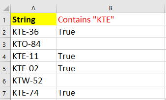
Ահա ապրանքի ID- ի ցուցակը, և այժմ ես ուզում եմ պարզել, թե արդյոք բջիջը պարունակում է «KTE» տող, և այնուհետև տեղադրել «TRUE» տեքստը դրա հարակից բջիջում, ինչպես ցույց է տրված նկարում: Այն լուծելու արագ ուղիներ ունե՞ք: Այս հոդվածում ես խոսում եմ հնարքների մասին `պարզելու, թե արդյոք բջիջը բառ է պարունակում, և ապա տեքստը հարակից խցում տեղադրելու համար:


Եթե ​​բջիջը բառ է պարունակում, ապա մեկ այլ բջիջ հավասար է որոշակի տեքստի

Ահա մի պարզ բանաձև, որը կարող է օգնել արագորեն ստուգել, ​​թե արդյոք բջիջը բառ է պարունակում, և ապա տեքստ տեղադրել դրա հաջորդ խցում:

Ընտրեք այն բջիջը, որը ցանկանում եք տեղադրել տեքստը և մուտքագրել այս բանաձևը = ԵԹԵ (ISNUMBER (Փնտրել ("KTE", A2)), "True", "") և ապա ավտոմատ լրացնելու բռնիչը ներքև քաշեք դեպի այն բջիջները, որոնք ցանկանում եք կիրառել այս բանաձևը: Տեսեք,

դոկ, եթե բջիջը բառ է պարունակում, ապա հավասար է 8-ի կրակոց նետը աջ դոկ, եթե բջիջը բառ է պարունակում, ապա հավասար է 9-ի


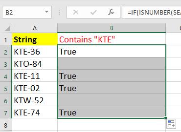
Բանաձևում A2- ը այն բջիջն է, որը ցանկանում եք ստուգել, ​​եթե պարունակում է որոշակի բառ, իսկ KTE- ն այն բառն է, որը ցանկանում եք ստուգել, ​​իսկականը այն տեքստն է, որը ցանկանում եք ցուցադրել մեկ այլ բջիջում: Կարող եք փոխել այս հղումները, որքան ձեզ հարկավոր է:


Եթե ​​բջիջը բառ է պարունակում, ապա ընտրեք կամ նշեք

Եթե ​​ցանկանում եք ստուգել, ​​արդյոք բջիջը պարունակում է որոշակի բառ, այնուհետև ընտրեք կամ ընդգծեք այն, կարող եք կիրառել այն Ընտրեք հատուկ բջիջներ առանձնահատկությունը Excel- ի համար նախատեսված գործիքներ, որը կարող է արագ կարգավորել այս աշխատանքը:

Excel- ի համար նախատեսված գործիքներ, ավելի քան 300 հարմար գործառույթներ, հեշտացնում է ձեր գործերը: 

Տեղադրելուց հետո Excel- ի համար նախատեսված գործիքներ, խնդրում ենք վարվել ինչպես ստորև :(Անվճար ներբեռնեք Kutools- ի համար Excel- ը հիմա!)

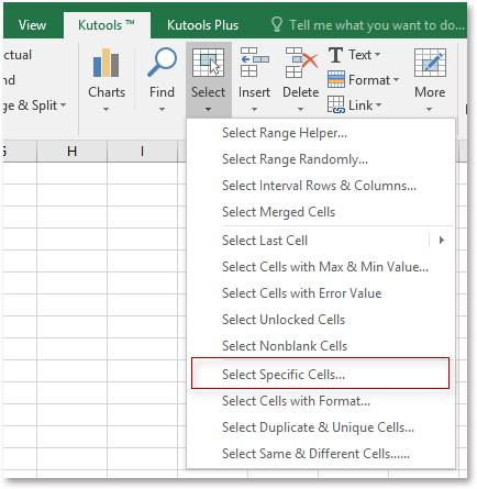
1. Ընտրեք այն տիրույթը, որը ցանկանում եք ստուգել, ​​արդյոք բջիջը որոշակի բառ է պարունակում, և կտտացրեք Կուտոլս > ընտրել > Ընտրեք հատուկ բջիջներ, Տեսեք,

դոկ, եթե բջիջը բառ է պարունակում, ապա հավասար է 3-ի

2. Դրանից հետո բացվող երկխոսության մեջ ստուգեք Բջիջ ընտրեք եւ ընտրեք Պարունակում է առաջին բացվող ցուցակից, ապա մուտքագրեք այն բառը, որը ցանկանում եք ստուգել հաջորդ տեքստային տուփի մեջ: Տեսեք,
դոկ, եթե բջիջը բառ է պարունակում, ապա հավասար է 4-ի

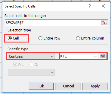
3: սեղմեք Ok, բացվում է երկխոսություն ՝ հիշեցնելու համար, թե ինչպես կարող են բջիջները պարունակել այն բառը, որը ցանկանում եք գտնել, և կտտացրեք OK երկխոսությունը փակելու համար: Տեսեք,
դոկ, եթե բջիջը բառ է պարունակում, ապա հավասար է 5-ի

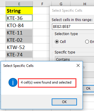
4. Դրանից հետո ընտրվել են նշված բառը պարունակող բջիջները, եթե ուզում եք դրանք ընդգծել, անցեք այստեղ Գլխավոր > Լրացրեք գույնը ընտրել մեկ լրացման գույն `դրանք առանձնացնելու համար:
դոկ, եթե բջիջը բառ է պարունակում, ապա հավասար է 6-ի

Հուշում Եթե ​​ցանկանում եք ունենալ անվճար փորձարկում Ընտրեք հատուկ բջիջներ գործառույթը, խնդրում ենք անցնել անվճար ներբեռնելու համար Kutools Excel- ի համար նախ և ապա անցեք գործողությունը կիրառելու համար ՝ համաձայն վերը նշված քայլերի:

Գրասենյակի արտադրողականության լավագույն գործիքները

🤖 Kutools AI օգնականՀեղափոխություն կատարել տվյալների վերլուծության հիման վրա՝ Խելացի կատարում   |  Ստեղծեք ծածկագիր  |  Ստեղծեք հատուկ բանաձևեր  |  Վերլուծել տվյալները և ստեղծել գծապատկերներ  |  Invoke Kutools-ի գործառույթները...
Հանրաճանաչ հատկություններ: Գտեք, ընդգծեք կամ նույնականացրեք կրկնօրինակները   |  Deleteնջել դատարկ շարքերը   |  Միավորել սյունակները կամ բջիջները՝ առանց տվյալների կորստի   |   Կլոր առանց բանաձևի ...
Super Փնտրել: Բազմաթիվ չափանիշների VLookup    Բազմակի արժեք VLookup  |   VLookup բազմաթիվ թերթերում   |   Fuzzy Փնտրել ....
Ընդլայնված բացվող ցուցակ: Արագ ստեղծեք բացվող ցուցակը   |  Կախված բացվող ցուցակ   |  Բազմակի ընտրություն Drop Down ցուցակ ....
Սյունակի կառավարիչ: Ավելացրեք որոշակի քանակությամբ սյունակներ  |  Տեղափոխել սյունակները  |  Փոխարկել թաքնված սյունակների տեսանելիության կարգավիճակը  |  Համեմատեք միջակայքերը և սյունակները ...
Առանձնահատկություններ: Ցանցի կենտրոնացում   |  Դիզայնի տեսք   |   Մեծ Formula Bar    Աշխատանքային գրքույկի և թերթիկների կառավարիչ   |  Ռեսուրսների գրադարան (Ավտոմատ տեքստ)   |  Ամսաթիվ ընտրող   |  Միավորել աշխատանքային թերթերը   |  Գաղտնագրել/գաղտնազերծել բջիջները    Ուղարկեք նամակներ ըստ ցանկի   |  Սուպեր զտիչ   |   Հատուկ զտիչ (զտել թավ/շեղ/շեղված...) ...
Լավագույն 15 գործիքների հավաքածու12 Տեքստ Գործիքներ (Ավելացրեք տեքստ, Հեռացնել նիշերը, ...)   |   50+ Աղյուսակ Տեսակներ (Գանտի աղյուսակը, ...)   |   40+ Գործնական Բանաձեւեր (Հաշվարկել տարիքը ՝ ելնելով ծննդյան տարեդարձից, ...)   |   19 միացում Գործիքներ (Տեղադրեք QR կոդ, Տեղադրեք նկար ուղուց, ...)   |   12 Փոխարկում Գործիքներ (Բառեր համարներ, Արտարժույթի փոխակերպումը, ...)   |   7 Միաձուլում և պառակտում Գործիքներ (Ընդլայնված կոմբինատ տողեր, Պառակտված բջիջներ, ...)   |   ... եւ ավելին

Լրացրեք ձեր Excel-ի հմտությունները Kutools-ի հետ Excel-ի համար և փորձեք արդյունավետությունը, ինչպես երբեք: Kutools-ը Excel-ի համար առաջարկում է ավելի քան 300 առաջադեմ առանձնահատկություններ՝ արտադրողականությունը բարձրացնելու և ժամանակ խնայելու համար:  Սեղմեք այստեղ՝ Ձեզ ամենաշատ անհրաժեշտ հատկանիշը ստանալու համար...

Նկարագրություն


Office Tab- ը Tabbed ինտերֆեյսը բերում է Office, և ձեր աշխատանքը շատ ավելի դյուրին դարձրեք

  • Միացնել ներդիրներով խմբագրումը և ընթերցումը Word, Excel, PowerPoint- ով, Հրատարակիչ, Access, Visio և Project:
  • Բացեք և ստեղծեք բազմաթիվ փաստաթղթեր նույն պատուհանի նոր ներդիրներում, այլ ոչ թե նոր պատուհաններում:
  • Բարձրացնում է ձեր արտադրողականությունը 50%-ով և նվազեցնում մկնիկի հարյուրավոր սեղմումները ձեզ համար ամեն օր:
Comments (21)
No ratings yet. Be the first to rate!
This comment was minimized by the moderator on the site
Buenas noches,

Tengo una columna con varias categorías de tareas (administrativo, profesor, etc) y quiero armar la columna siguiente indicando si es x tarea que sea nivel alto, si es otra Medio y así. Intenté con la fórmula SI y SI. CONJUNTO pero no parece funcionar cuando no hay valores numéricos. Vi ejemplos pero con si C2 es mayor que entonces tal palabra...
This comment was minimized by the moderator on the site
Buen día, disculpa, queria ver si me puedes ayudar con una formula.

En una celda tengo una oracion, y quiero que la celda de un lado me escriba cierta letra o palabra cuando en la primera celda tenga alguna palabra.

Ejemplo
en la celda A1 tengo una oracion: papa manzana pasta, lechuga.
en la celda A2 tengo: papa manzana, zanahoria, lechuga.

Quiero que en la celda B1 me aparezca la palabra "ensalada" solo porque en la A1 tiene "lechuga"
y en la celda B2 me aparezca la palabra: "arbol" porque tiene la palabra "manzana"

Nota quiero que de prioridad a la lechuga antes que a la manzana
Sino se puede dar prioridad entonces digamos que quitamos la palabra "manzana" de la primera oracion


No se si me di a entender, no se me ocurrio como dar el ejemplo
This comment was minimized by the moderator on the site
Hi, luis, here is a formula may help you.
Take an example for explaining the formula, if cell contains "KTE" then returns "Y", if cell contains "KTW" then returns "T", if cell contains both of "KTE' and "KTW" then returns "Y".
=IF(AND(ISNUMBER(SEARCH("KTE",A3)), ISNUMBER(SEARCH("KTW",A3)) ),"Y", IF(ISNUMBER(SEARCH("KTE",A3)), "Y", IF(ISNUMBER(SEARCH("KTW",A3)), "T", "")))
change the reference and the values as you need.
https://www.extendoffice.com/images/stories/comments/sun-comment/doc-return-value-based-on-word.png
Tip: If you in spanish version, maybe need to change the formula to spanish formula.
This comment was minimized by the moderator on the site
How do you keep this going, if I have 5 other unique labels that need to spit out 5 other unique corresponding phrases?
This comment was minimized by the moderator on the site
Hi, Andy, yes, you need to use 5 different formulas to acheive your purpose.
This comment was minimized by the moderator on the site
kolom satu
adam
andi
budi
dst

kolom dua
andi jaya
budiarto
adam malik
dst


kolom 3 (hasil pakai rumus)


pertanyaan:
bagaimana rumus di kolom 3, jika kita ingin memunculkan nama kolom 2 dikolom 3 yg mengandung teks di kolom satu.

saya minta petunjuk dari para pakar excel.

Terima kasih
Andi
This comment was minimized by the moderator on the site
Hi, Andi, I realy like to help you, but I cannot read your language, could you login and upload a screenshot to show the result you want? Then I will try to find method to solve it.
This comment was minimized by the moderator on the site
kolom satu kolom dua kolom 3 (hasil rumus)
adam andi jaya
andi budiarto
budi adam malik
dst dst

bagaimana rumus di kolom 3, jika kita ingin memunculkan nama kolom 2 dikolom 3 yg mengandung teks di kolom satu.

saya minta petunjuk dari para pakar excel.

Terima kasih
Andi
This comment was minimized by the moderator on the site
If column has text, alpha-numeric & numeric values, using the convert tool does not apply the text values to numeric. Makes sense. Though, how could you configure a IF Vlookup to compensate if a cell has text?
This comment was minimized by the moderator on the site
Sorry, which convert tool you mean? The formula can work correctly whatever the column contains alpha, alpha-numeric or numeric string.
This comment was minimized by the moderator on the site
Hello,

Question. If I need this formula to apply to two different returns. For example, if a cell contains the word "Senior", another cell would return "32" and if the cell contains "Associate" then the other cell would return 16.
This comment was minimized by the moderator on the site
Here's the formula. Assume there's a list of titles starting in cell A2:

Senior Engineer
Associate Engineer
Senior Engineer
Senior Engineer
Vice President
Associate Engineer
Associate Engineer
Senior Vice Presdent

In cell B2 (or whatever cell you wish to populate with the results), write:

=IF(ISNUMBER(FIND("Senior",A2)),"32",IF(ISNUMBER(FIND("Associate",A2)),"16"))

You could check for additional values by adding additional nested IF statements.
This comment was minimized by the moderator on the site
Sorry I cannot figore out the correct formula to solve your problem, you can go to our forum https://www.extendoffice.com/forum.html to place your question, maybe someone can help you.
This comment was minimized by the moderator on the site
Thanks for this. Can this code be edited so that instead of placing specific text beside the source text, it can be formatted to place the text in a different cell?
This comment was minimized by the moderator on the site
i know what u mean. i need this function to.
This comment was minimized by the moderator on the site
Do you mean to extract the text in different cell while the cell contains the specifict text as below screenshot shown?
This comment was minimized by the moderator on the site
Sorry, I do not realy understand your question. Could you give me more detail description?
This comment was minimized by the moderator on the site
How would you write the formula is you have text-text-text and you want to pull the final text? AB-GUFJ-CD if you want to pull the CD?
This comment was minimized by the moderator on the site
Hello, this formula may help you =TRIM(RIGHT(SUBSTITUTE(A12,"-",REPT(" ",255)),255)), A12 is the text string you use, change it as you need. If it works, please let me know. Thanks.
This comment was minimized by the moderator on the site
LOL ...did you mean True?
This comment was minimized by the moderator on the site
Embarrrassed...yes, I mean true~~, I have rewrote it, thank u for ur remind.
There are no comments posted here yet
Please leave your comments in English
Posting as Guest
×
Rate this post:
0   Characters
Suggested Locations