Բաց թողնել հիմնական բովանդակությունը

Ինչպե՞ս գտնել Excel- ում n- ի ոչ դատարկ բջիջը:

Հեղինակ՝ Սյաոյանգ Վերջին փոփոխությունը՝ 2020-07-03

Ինչպե՞ս կարող եք գտնել և վերադարձնել Excel- ի սյունակից կամ տողից n- ի ոչ դատարկ բջիջի արժեքը: Այս հոդվածում ես կխոսեմ այս խնդիրը լուծելու համար ձեզ համար օգտակար բանաձևերի մասին:

Բանաձևով սյունակից գտեք և վերադարձրեք n- ի ոչ դատարկ բջիջի արժեքը

Գտեք և վերադարձեք բանաձևով շարքից տասներորդ ոչ դատարկ բջիջի արժեքը


նետ կապույտ աջ պղպջակ Բանաձևով սյունակից գտեք և վերադարձրեք n- ի ոչ դատարկ բջիջի արժեքը

Օրինակ, ես ունեմ տվյալների սյուն, ինչպես ցույց է տրված հետևյալ նկարը, այժմ ես այս ցուցակից կստանամ երրորդ ոչ դատարկ բջիջի արժեքը:

doc գտնել nth ոչ դատարկ 1

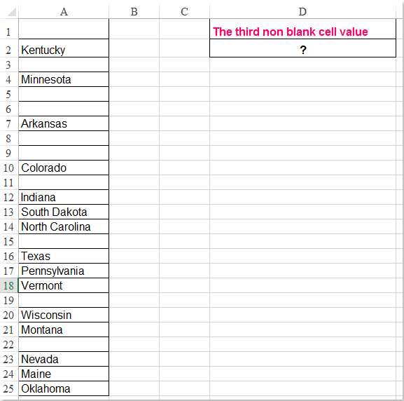
Խնդրում ենք մուտքագրել այս բանաձևը. =INDEX($A$1:$A$25,SMALL(ROW($A$1:$A$25)+(100*($A$1:$A$25="")), 3))&"" դատարկ բջիջի մեջ, որտեղ ցանկանում եք արդյունքը դուրս բերել, օրինակ, D2, ապա սեղմել Ctrl + Shift + Մուտք ստեղները միասին ՝ ճիշտ արդյունք ստանալու համար, տես նկարի նկարը.

doc գտնել nth ոչ դատարկ 2

ՆշումՎերը նշված բանաձևում A1: A25 տվյալների ցանկն է, որը ցանկանում եք օգտագործել և համարը 3 նշում է երրորդ ոչ դատարկ բջիջի արժեքը, որը ցանկանում եք վերադարձնել, եթե ուզում եք ստանալ երկրորդ ոչ դատարկ բջիջը, պարզապես անհրաժեշտ է փոխել 3-ը 2-ի համարը, որքան ձեզ հարկավոր է:


նետ կապույտ աջ պղպջակ Գտեք և վերադարձեք բանաձևով շարքից տասներորդ ոչ դատարկ բջիջի արժեքը

Եթե ​​ցանկանում եք անընդմեջ գտնել և վերադարձնել n- ի ոչ դատարկ բջիջի արժեքը, հետևյալ բանաձևը կարող է օգնել ձեզ, խնդրում ենք արեք հետևյալ կերպ.

Մուտքագրեք այս բանաձևը. =INDEX($A$1:$M$1,SMALL(IF($A$1:$M$1<>"",COLUMN($A$1:$M$1)-COLUMN($A$1)+1),4)) դատարկ բջիջի մեջ, որտեղ ցանկանում եք գտնել արդյունքը, ապա սեղմել Ctrl + Shift + Մուտք ստեղները միասին ՝ արդյունքը ստանալու համար, տես նկարի նկարը.

doc գտնել nth ոչ դատարկ 3

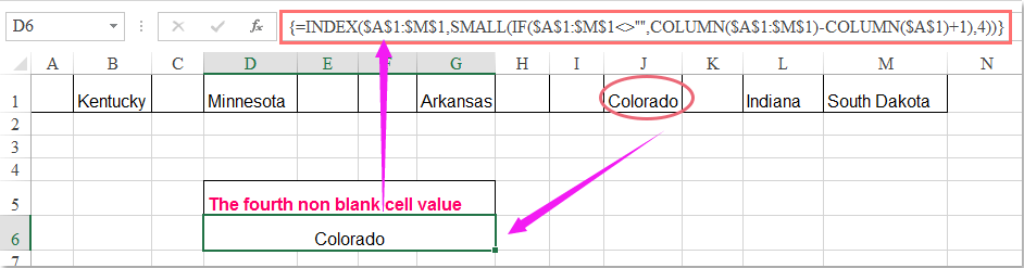
Նշում: Վերոնշյալ բանաձևում A1: M1 տողի արժեքներն են, որոնք ցանկանում եք օգտագործել, և համարը 4 չորրորդ ոչ դատարկ բջիջի արժեքն է, որը ցանկանում եք վերադարձնել, եթե ցանկանում եք ստանալ երկրորդ ոչ դատարկ բջիջը, պարզապես անհրաժեշտ է փոխել 4-ը 2-ի համարը, որքան ձեզ հարկավոր է:

Գրասենյակի արտադրողականության լավագույն գործիքները

🤖 Kutools AI օգնականՀեղափոխություն կատարել տվյալների վերլուծության հիման վրա՝ Խելացի կատարում   |  Ստեղծեք ծածկագիր  |  Ստեղծեք հատուկ բանաձևեր  |  Վերլուծել տվյալները և ստեղծել գծապատկերներ  |  Invoke Kutools-ի գործառույթները...
Հանրաճանաչ հատկություններ: Գտեք, ընդգծեք կամ նույնականացրեք կրկնօրինակները   |  Deleteնջել դատարկ շարքերը   |  Միավորել սյունակները կամ բջիջները՝ առանց տվյալների կորստի   |   Կլոր առանց բանաձևի ...
Super Փնտրել: Բազմաթիվ չափանիշների VLookup    Բազմակի արժեք VLookup  |   VLookup բազմաթիվ թերթերում   |   Fuzzy Փնտրել ....
Ընդլայնված բացվող ցուցակ: Արագ ստեղծեք բացվող ցուցակը   |  Կախված բացվող ցուցակ   |  Բազմակի ընտրություն Drop Down ցուցակ ....
Սյունակի կառավարիչ: Ավելացրեք որոշակի քանակությամբ սյունակներ  |  Տեղափոխել սյունակները  |  Փոխարկել թաքնված սյունակների տեսանելիության կարգավիճակը  |  Համեմատեք միջակայքերը և սյունակները ...
Առանձնահատկություններ: Ցանցի կենտրոնացում   |  Դիզայնի տեսք   |   Մեծ Formula Bar    Աշխատանքային գրքույկի և թերթիկների կառավարիչ   |  Ռեսուրսների գրադարան (Ավտոմատ տեքստ)   |  Ամսաթիվ ընտրող   |  Միավորել աշխատանքային թերթերը   |  Գաղտնագրել/գաղտնազերծել բջիջները    Ուղարկեք նամակներ ըստ ցանկի   |  Սուպեր զտիչ   |   Հատուկ զտիչ (զտել թավ/շեղ/շեղված...) ...
Լավագույն 15 գործիքների հավաքածու12 Տեքստ Գործիքներ (Ավելացրեք տեքստ, Հեռացնել նիշերը, ...)   |   50+ Աղյուսակ Տեսակներ (Գանտի աղյուսակը, ...)   |   40+ Գործնական Բանաձեւեր (Հաշվարկել տարիքը ՝ ելնելով ծննդյան տարեդարձից, ...)   |   19 միացում Գործիքներ (Տեղադրեք QR կոդ, Տեղադրեք նկար ուղուց, ...)   |   12 Փոխարկում Գործիքներ (Բառեր համարներ, Արտարժույթի փոխակերպումը, ...)   |   7 Միաձուլում և պառակտում Գործիքներ (Ընդլայնված կոմբինատ տողեր, Պառակտված բջիջներ, ...)   |   ... եւ ավելին

Լրացրեք ձեր Excel-ի հմտությունները Kutools-ի հետ Excel-ի համար և փորձեք արդյունավետությունը, ինչպես երբեք: Kutools-ը Excel-ի համար առաջարկում է ավելի քան 300 առաջադեմ առանձնահատկություններ՝ արտադրողականությունը բարձրացնելու և ժամանակ խնայելու համար:  Սեղմեք այստեղ՝ Ձեզ ամենաշատ անհրաժեշտ հատկանիշը ստանալու համար...

Նկարագրություն


Office Tab- ը Tabbed ինտերֆեյսը բերում է Office, և ձեր աշխատանքը շատ ավելի դյուրին դարձրեք

  • Միացնել ներդիրներով խմբագրումը և ընթերցումը Word, Excel, PowerPoint- ով, Հրատարակիչ, Access, Visio և Project:
  • Բացեք և ստեղծեք բազմաթիվ փաստաթղթեր նույն պատուհանի նոր ներդիրներում, այլ ոչ թե նոր պատուհաններում:
  • Բարձրացնում է ձեր արտադրողականությունը 50%-ով և նվազեցնում մկնիկի հարյուրավոր սեղմումները ձեզ համար ամեն օր:
Comments (10)
No ratings yet. Be the first to rate!
This comment was minimized by the moderator on the site
CIAO STO CERCANDO DI APPLICARE LA TUA FORMULA MA NON MI FUNZIONA, DOVE STO SBAGLIANDO?
=INDICE($K$37:$K$88;MIN(RIGHE($K$37:$K$88)+RIGHE(100*($K$37:$K$88=""));6))&""
DEVO VISUALIZZARE L'ENNESIMA RIGA DIVERSA DA VUOTO

GRAzie
This comment was minimized by the moderator on the site
=INDICE($K$37:$K$88;MIN(RIGHE($K$37:$K$88)+(100*($K$37:$K$88=""));6))&""
This comment was minimized by the moderator on the site
I'm running this formula on a ~400 row sheet with around 20 blanks mixed throughout the data, and it's working perfectly EXCEPT when I fill the series down, it sometimes duplicates a row for some reason. For example, it seems to think a value is somehow simultaneously the 331st non-blank and the 332nd.

Things I've noticed:
-Duplications always happen in pairs (ex. 331 and 332 are duplicates, 333 and 334 will also be), then it goes back to normal for a while.
-Raw data also has blanks in pairs, but not corresponding to the duplicates
-No duplications occur in the first 94 rows, but they happen every 33-35 rows after that
-Does not appear to be linked to the value in the cell being duplicated
-I have entered as an array and as a standard formula, no difference in function

For reference, here's my actual formula:

=INDEX('PO Raw Data'!CR:CR,SMALL(ROW('PO Raw Data'!CR:CR)+(100*('PO Raw Data'!CR:CR="")),$W2)&"")

Note $W2 refers to a helper column and counts up as the data set is filled down, but only because I couldn't get it to count up when I just used a number instead of cell reference.
When I've replaced that cell reference (ex. $W2) with the appropriate number, same result.


Any thoughts on what I can do to fix that?
This comment was minimized by the moderator on the site
very helpful,
although when I return the nth non blank cell in a column set to DATE, the returned value appears as number(general number).formatting the cell into DATE also doesn't change the result. could you please give me a hand!
thanks a lot
This comment was minimized by the moderator on the site
Hello, Shirazi,
Sorry, maybe there is no direct formula for you to get the date format.

If someone else has the solution, please comment here.
This comment was minimized by the moderator on the site
Hi everyone!


Could you also help me return the row number of the second, third non-blank cell?


Please help me.
This comment was minimized by the moderator on the site
Hello, John,
the following formula can help you to get all the row numbers of the non-blank cells, please try it, thank you!
=IFERROR(ROW(INDEX($A$1:$A$12,SMALL(INDEX(NOT(ISBLANK($A$1:$A$12))*ROW($A$1:$A$12),0),COUNTBLANK($A$1:$A$12)+ROW(A1)))),"")
This comment was minimized by the moderator on the site
Hey everyone,

I have a table with numerous columns and rows. The rows have range names, and a description/location at the beginning of the row range with its own range, example "Building No.s". There are multiple Row Ranges/ Buildings. There are headers at the top of each columns for specific "Building Assembly Types". The table content is numeric quantities for each type "Building Assembly Type" for each specific "Building" description/location. There could be as many as (100) "Building Assembly Types" column headers but I will limit the assemblies to (10) per row range, so there will be numerous blank cells in each "Building No." range.

I have other summary tables set up for each "Building" that I want to pull the non-blank cells quantities to, along with the corresponding header "Assembly Type" for each "Building" with a (10) max "Assemblies" per page.

I can identify the non-blank cell quantities by use of the array formula above for rows. The problem I am having is identifying the header that corresponds to it.

Ultimately if I can identify the "Assembly" header, I can always index the "Quantities" once I have the header "Assembly" identified for each "Building". Then I would be able do a lookup for all the parts associated with each "Assembly" type for that "Building" from my Assembly parts database and multiply it times the "Quantity" of each assembly type.

Hopefully this makes since and someone can help.
This comment was minimized by the moderator on the site
Hello, I am looking for the third blank row in a column and I copied your formula and just changed the range from $A$1:$A:$25 to my range $D$306:$D$354. But when I change the range I get #REF! as my answer. I already converted to an array, control-shift-enter. Now the cell range I am referencing has formulas in them, so could that be why I am getting #REF. Your formula: =INDEX($A$1:$A$25,SMALL(ROW($A$1:$A$25)+(100*($A$1:$A$25="")), 3))&"" My formula: =INDEX($D$306:$D$354,SMALL(ROW($D$306:$D$354)+(1*($D$306:$D$354="")), 2))&"" Thanks, Noel
This comment was minimized by the moderator on the site
you have put the 1 instead of 100 therefore answered was wrong. please use below formula

INDEX($D$306:$D$354,SMALL(ROW($D$306:$D$354)+(100*($D$306:$D$354="")), 3))&"" than ctrl + shift+enter
There are no comments posted here yet
Please leave your comments in English
Posting as Guest
×
Rate this post:
0   Characters
Suggested Locations