Բաց թողնել հիմնական բովանդակությունը

Ինչպե՞ս VLOOKUP- ը և հորիզոնական վերադարձնել բազմաթիվ համապատասխան արժեքներ Excel- ում:

doc-vlookup-horizontal-1
Լռելյայնորեն, VLOOKUP գործառույթը կարող է Excel- ում ուղղահայաց մակարդակում վերադարձնել բազմաթիվ համապատասխան արժեքներ, որոշ դեպքերում կարող է ցանկանալ վերադարձնել բազմաթիվ արժեքներ հորիզոնական մակարդակում, ինչպես ցույց է տրված նկարում: Այստեղ ես ձեզ կասեմ, որ բանաձևը կարող է լուծել այս խնդիրը:
VLOOKUP- ը և հորիզոնական վերադարձնել բազմաթիվ արժեքներ

նետ կապույտ աջ պղպջակ VLOOKUP- ը և հորիզոնական վերադարձնել բազմաթիվ արժեքներ

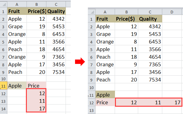
Օրինակ, դուք ունեք տվյալների մի շարք, ինչպես ցույց է տրված ստորև նշված էկրանի նկարը, և ցանկանում եք VLOOKUP- ը Apple- ի գները:
doc-vlookup-horizontal-2

1. Ընտրեք բջիջ և մուտքագրեք այս բանաձևը =INDEX($B$2:$B$9, SMALL(IF($A$11=$A$2:$A$9, ROW($A$2:$A$9)-ROW($A$2)+1), COLUMN(A1))) մտեք դրան, ապա սեղմեք Shift + Ctrl + Enter և քաշեք ինքնալրացման բռնիչը աջ ՝ այս բանաձևը կիրառելու համար մինչև # ԱՆUM! հայտնվում է. Տեսեք,
doc-vlookup-horizontal-3

2. Ապա ջնջեք #NUM- ը: Տեսեք,
doc-vlookup-horizontal-4

Ձեր պատասխանը ուղարկված չէ: Վերոնշյալ բանաձևում B2: B9- ը սյունակի տիրույթ է, որում ցանկանում եք վերադարձնել արժեքները, A2: A9- ը սյունակի տիրույթ է, որի մեջ գտնվում է որոնման արժեքը, A11- ը որոնման արժեք է, A1- ը ՝ ձեր տվյալների տիրույթի առաջին բջիջը , A2- ը սյունակի տիրույթի առաջին բջիջն է, որի մեջ որոնման արժեքը գտնվում է:

Եթե ​​ցանկանում եք ուղղահայաց վերադարձնել բազմաթիվ արժեքներ, կարող եք կարդալ այս հոդվածը Ինչպե՞ս որոնել արժեքը Excel- ում մի քանի համապատասխան արժեքներ վերադարձնելու համար:


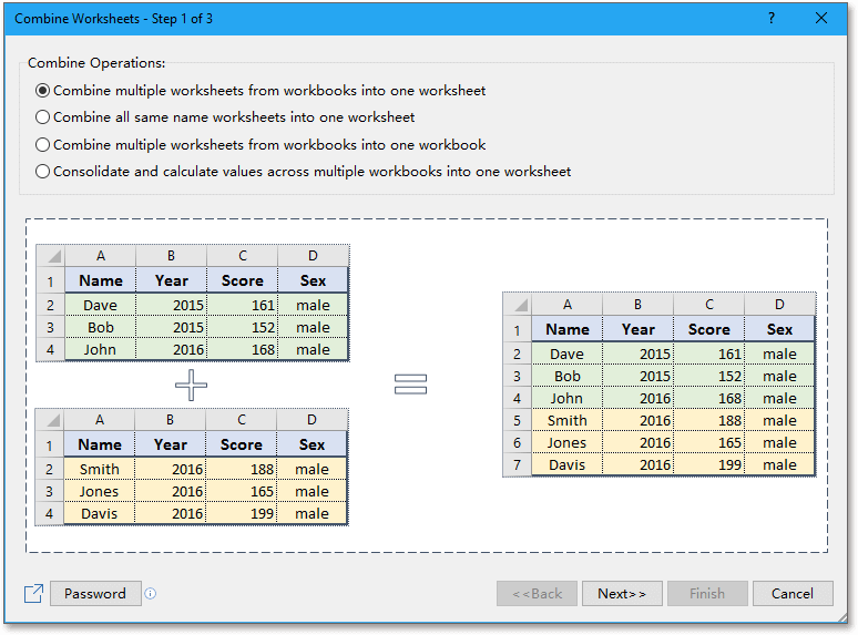
Հեշտությամբ միացրեք մի քանի թերթ / աշխատանքային գրքույկ մեկ եզակի թերթի կամ աշխատանքային գրքի մեջ

Բազմապատկերի թերթերը կամ աշխատանքային գրքերը մեկ թերթիկի կամ աշխատանքային գրքի մեջ միավորելը Excel- ում կարող է համառ լինել, բայց հետևյալով Միավորել գործառույթ Kutools- ում Excel- ի համար, դուք կարող եք միավորել տասնյակ թերթեր / աշխատանքային գրքեր մեկ թերթիկի կամ աշխատանքային գրքի մեջ, ինչպես նաև կարող եք միավորել թերթերը միայն մեկ կտտոցով:  Կտտացրեք լիարժեք 30 օր անվճար փորձաշրջանի համար:
համատեղել սավանները
 
Excel- ի համար նախատեսված գործիքներ. Ավելի քան 300 հարմար Excel հավելվածներով, 30 օրում առանց սահմանափակումների անվճար փորձեք:

Գրասենյակի արտադրողականության լավագույն գործիքները

🤖 Kutools AI օգնականՀեղափոխություն կատարել տվյալների վերլուծության հիման վրա՝ Խելացի կատարում   |  Ստեղծեք ծածկագիր  |  Ստեղծեք հատուկ բանաձևեր  |  Վերլուծել տվյալները և ստեղծել գծապատկերներ  |  Invoke Kutools-ի գործառույթները...
Հանրաճանաչ հատկություններ: Գտեք, ընդգծեք կամ նույնականացրեք կրկնօրինակները   |  Deleteնջել դատարկ շարքերը   |  Միավորել սյունակները կամ բջիջները՝ առանց տվյալների կորստի   |   Կլոր առանց բանաձևի ...
Super Փնտրել: Բազմաթիվ չափանիշների VLookup    Բազմակի արժեք VLookup  |   VLookup բազմաթիվ թերթերում   |   Fuzzy Փնտրել ....
Ընդլայնված բացվող ցուցակ: Արագ ստեղծեք բացվող ցուցակը   |  Կախված բացվող ցուցակ   |  Բազմակի ընտրություն Drop Down ցուցակ ....
Սյունակի կառավարիչ: Ավելացրեք որոշակի քանակությամբ սյունակներ  |  Տեղափոխել սյունակները  |  Փոխարկել թաքնված սյունակների տեսանելիության կարգավիճակը  |  Համեմատեք միջակայքերը և սյունակները ...
Առանձնահատկություններ: Ցանցի կենտրոնացում   |  Դիզայնի տեսք   |   Մեծ Formula Bar    Աշխատանքային գրքույկի և թերթիկների կառավարիչ   |  Ռեսուրսների գրադարան (Ավտոմատ տեքստ)   |  Ամսաթիվ ընտրող   |  Միավորել աշխատանքային թերթերը   |  Գաղտնագրել/գաղտնազերծել բջիջները    Ուղարկեք նամակներ ըստ ցանկի   |  Սուպեր զտիչ   |   Հատուկ զտիչ (զտել թավ/շեղ/շեղված...) ...
Լավագույն 15 գործիքների հավաքածու12 Տեքստ Գործիքներ (Ավելացրեք տեքստ, Հեռացնել նիշերը, ...)   |   50+ Աղյուսակ Տեսակներ (Գանտի աղյուսակը, ...)   |   40+ Գործնական Բանաձեւեր (Հաշվարկել տարիքը ՝ ելնելով ծննդյան տարեդարձից, ...)   |   19 միացում Գործիքներ (Տեղադրեք QR կոդ, Տեղադրեք նկար ուղուց, ...)   |   12 Փոխարկում Գործիքներ (Բառեր համարներ, Արտարժույթի փոխակերպումը, ...)   |   7 Միաձուլում և պառակտում Գործիքներ (Ընդլայնված կոմբինատ տողեր, Պառակտված բջիջներ, ...)   |   ... եւ ավելին

Լրացրեք ձեր Excel-ի հմտությունները Kutools-ի հետ Excel-ի համար և փորձեք արդյունավետությունը, ինչպես երբեք: Kutools-ը Excel-ի համար առաջարկում է ավելի քան 300 առաջադեմ առանձնահատկություններ՝ արտադրողականությունը բարձրացնելու և ժամանակ խնայելու համար:  Սեղմեք այստեղ՝ Ձեզ ամենաշատ անհրաժեշտ հատկանիշը ստանալու համար...

Նկարագրություն


Office Tab- ը Tabbed ինտերֆեյսը բերում է Office, և ձեր աշխատանքը շատ ավելի դյուրին դարձրեք

  • Միացնել ներդիրներով խմբագրումը և ընթերցումը Word, Excel, PowerPoint- ով, Հրատարակիչ, Access, Visio և Project:
  • Բացեք և ստեղծեք բազմաթիվ փաստաթղթեր նույն պատուհանի նոր ներդիրներում, այլ ոչ թե նոր պատուհաններում:
  • Բարձրացնում է ձեր արտադրողականությունը 50%-ով և նվազեցնում մկնիկի հարյուրավոր սեղմումները ձեզ համար ամեն օր:
Comments (20)
No ratings yet. Be the first to rate!
This comment was minimized by the moderator on the site
This article says this uses VLOOKUP, but it uses INDEX... which does not help me. I need a solution for multiple values using VLOOKUP or XLOOKUP in tables.
This comment was minimized by the moderator on the site
you can use TEXTSPLIT function followed by TEXTJOIN FUNCTION in excel 365
This comment was minimized by the moderator on the site
For anyone experiencing issues in a big data range, ensure you dont have any cells existent with "#N/A" or it will break it. Simple error but can be overlooked.
This comment was minimized by the moderator on the site
Hello, I want to use keyword instead of specific text or value here for multiple return values, can you please share code formula for same.
This comment was minimized by the moderator on the site
Hello - This formula worked perfectly - thank you! However, I want to apply it to a long list of lookup values. When I copy and paste the formula it obviously returns the same results as the first lookup value so I removed the $'s from $A$11, but that changes the result to something incorrect. How can I quickly apply this same formula for a long list of lookup values?

Thank you!

M
This comment was minimized by the moderator on the site
Bonjour,

J'ai retransposé mon problème exactement dans les mêmes positions de colonne que l'exemple et j’obtiens le message #VALEUR! dès la première case.

Mon excel fonctionne en francais, j'ai tout retranscrit en francais, passé ";"au lieu de ",", appuyé sur CTRL+MAJ+Entrée... des idées sur l'origine du problème?

Fanny
This comment was minimized by the moderator on the site
what you want to put the price in order of highest qty from column c?
This comment was minimized by the moderator on the site
i have to find vertical value first, in vertical value there are more horizontal value and i have choose grater value which i have. which function or formula can help
This comment was minimized by the moderator on the site
Hi. I have three google spreadsheet. First sheet is named "Summary. It is a table containing the name of our employee and number of evaluation in a week from 1-7. The next sheet is named "Chat Score"and third sheet is named Ëmail Score". What I want to to do is when we input a evaluation score to one of our employee it will be automatically recorded on the "Summary sheet" as evaluation 1 or 2 and so on and so forth. In short I want to get multiple return value in a single seach key across multiple sheet. I hope you can help. https://docs.google.com/spreadsheets/d/1lt-e4MxddUKg5xDt_0YchBiEgGe4mFKB-dHENwwtA6Y/edit?usp=sharing

https://docs.google.com/spreadsheets/d/1lt-e4MxddUKg5xDt_0YchBiEgGe4mFKB-dHENwwtA6Y/edit?usp=sharing
This comment was minimized by the moderator on the site
Although I'm looking up my values in another worksheet (I don't think this should cause a problem?), I only seem to have success dragging to the right if I go in and change the +1 to '0' for the 1st instance of the lookup ID, '1' for the 2nd instance and so on. I know how many instances of the lookup ID I have so I can workaround. What do I need to change to allow me to successfully drag the fx across horizontally without needing to edit (i.e getting the #NUM to appear once there are no more lookup values to return).
This comment was minimized by the moderator on the site
Sorry, I have not found any solutions about your problems. If you have found that, could you tell me? Thank u.
This comment was minimized by the moderator on the site
Change Column to Row at the end of the formula

"=INDEX($B$1:$B$206, SMALL(IF($A$209=$A$1:$A$206, ROW($A$1:$A$206)-ROW($A$1)+1), ROW(A1)))"
This comment was minimized by the moderator on the site
How to List all values(like list of groceries bought) caused by a specific value (by a person X) using VLOOK_UP and other possible formulas
This comment was minimized by the moderator on the site
You mean that to list all grocerise a person need to buy, right? If so, you can refer to the formula in this article, and change the arguments as you need as below screenshot shown.
There are no comments posted here yet
Load More
Please leave your comments in English
Posting as Guest
×
Rate this post:
0   Characters
Suggested Locations