Բաց թողնել հիմնական բովանդակությունը

Ինչպե՞ս Excel- ում բջջային գույնը հավասարեցնել բջջի մեկ այլ գույնի:

Հեղինակ՝ Սիլյուվիա Վերջին փոփոխությունը՝ 2020-06-17

Եթե ​​ցանկանում եք բջջի գույնը համապատասխանեցնել մեկ այլ գույնի, ապա այս հոդվածի մեթոդը կարող է օգնել ձեզ:

Սահմանեք բջիջի գույնը հավասար մեկ այլ բջիջի գույնի VBA կոդով


Սահմանեք բջիջի գույնը հավասար մեկ այլ բջիջի գույնի VBA կոդով

Ստորև ներկայացված VBA մեթոդը կարող է օգնել Excel- ում մեկ այլ բջիջի հավասար գույն ընտրել: Խնդրում եմ, արեք հետևյալ կերպ.

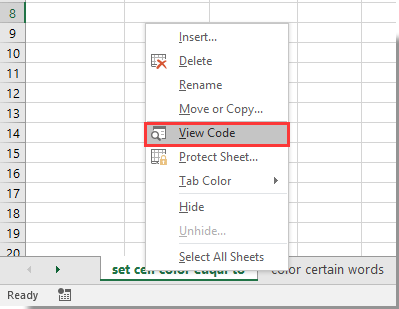
1. Աշխատաթերթում անհրաժեշտ է երկու բջիջների գույնը համապատասխանեցնել, խնդրում ենք աջ կտտացնել թերթիկի ներդիրին և այնուհետև կտտացնել Դիտել կոդը աջ կտտացնելու ցանկից: Տեսեք,

2. Բացման մեջ Microsoft Visual Basic հավելվածների համար պատուհան, դուք պետք է պատճենեք և կպցրեք VBA կոդը օրենսգրքի պատուհանում:

VBA կոդ. Բջջի գույնը սահմանիր բջջի մեկ այլ գույնի հավասար

Private Sub Worksheet_SelectionChange(ByVal Target As Range)
    Me.Range("C1").Interior.Color = Me.Range("A1").Interior.Color
End Sub

ՆշումԿոդում `A1- ն այն բջիջն է, որը պարունակում է լրացման գույն, որը կհամապատասխանես C1- ի: Խնդրում ենք փոխել դրանք ՝ ելնելով ձեր կարիքներից:

Դրանից հետո C1 բջիջը լցվում է նույն գույնի A1 բջիջով, ինչպես ցույց է տրված նկարում:

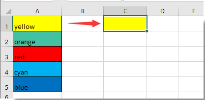
Այսուհետ, երբ A1- ի լրացման գույնը փոխվում է, C1- ը ավտոմատ կերպով կհամընկնի նույն գույնի հետ:


Առնչվող հոդվածներ քանակը:

Գրասենյակի արտադրողականության լավագույն գործիքները

🤖 Kutools AI օգնականՀեղափոխություն կատարել տվյալների վերլուծության հիման վրա՝ Խելացի կատարում   |  Ստեղծեք ծածկագիր  |  Ստեղծեք հատուկ բանաձևեր  |  Վերլուծել տվյալները և ստեղծել գծապատկերներ  |  Invoke Kutools-ի գործառույթները...
Հանրաճանաչ հատկություններ: Գտեք, ընդգծեք կամ նույնականացրեք կրկնօրինակները   |  Deleteնջել դատարկ շարքերը   |  Միավորել սյունակները կամ բջիջները՝ առանց տվյալների կորստի   |   Կլոր առանց բանաձևի ...
Super Փնտրել: Բազմաթիվ չափանիշների VLookup    Բազմակի արժեք VLookup  |   VLookup բազմաթիվ թերթերում   |   Fuzzy Փնտրել ....
Ընդլայնված բացվող ցուցակ: Արագ ստեղծեք բացվող ցուցակը   |  Կախված բացվող ցուցակ   |  Բազմակի ընտրություն Drop Down ցուցակ ....
Սյունակի կառավարիչ: Ավելացրեք որոշակի քանակությամբ սյունակներ  |  Տեղափոխել սյունակները  |  Փոխարկել թաքնված սյունակների տեսանելիության կարգավիճակը  |  Համեմատեք միջակայքերը և սյունակները ...
Առանձնահատկություններ: Ցանցի կենտրոնացում   |  Դիզայնի տեսք   |   Մեծ Formula Bar    Աշխատանքային գրքույկի և թերթիկների կառավարիչ   |  Ռեսուրսների գրադարան (Ավտոմատ տեքստ)   |  Ամսաթիվ ընտրող   |  Միավորել աշխատանքային թերթերը   |  Գաղտնագրել/գաղտնազերծել բջիջները    Ուղարկեք նամակներ ըստ ցանկի   |  Սուպեր զտիչ   |   Հատուկ զտիչ (զտել թավ/շեղ/շեղված...) ...
Լավագույն 15 գործիքների հավաքածու12 Տեքստ Գործիքներ (Ավելացրեք տեքստ, Հեռացնել նիշերը, ...)   |   50+ Աղյուսակ Տեսակներ (Գանտի աղյուսակը, ...)   |   40+ Գործնական Բանաձեւեր (Հաշվարկել տարիքը ՝ ելնելով ծննդյան տարեդարձից, ...)   |   19 միացում Գործիքներ (Տեղադրեք QR կոդ, Տեղադրեք նկար ուղուց, ...)   |   12 Փոխարկում Գործիքներ (Բառեր համարներ, Արտարժույթի փոխակերպումը, ...)   |   7 Միաձուլում և պառակտում Գործիքներ (Ընդլայնված կոմբինատ տողեր, Պառակտված բջիջներ, ...)   |   ... եւ ավելին

Լրացրեք ձեր Excel-ի հմտությունները Kutools-ի հետ Excel-ի համար և փորձեք արդյունավետությունը, ինչպես երբեք: Kutools-ը Excel-ի համար առաջարկում է ավելի քան 300 առաջադեմ առանձնահատկություններ՝ արտադրողականությունը բարձրացնելու և ժամանակ խնայելու համար:  Սեղմեք այստեղ՝ Ձեզ ամենաշատ անհրաժեշտ հատկանիշը ստանալու համար...

Նկարագրություն


Office Tab- ը Tabbed ինտերֆեյսը բերում է Office, և ձեր աշխատանքը շատ ավելի դյուրին դարձրեք

  • Միացնել ներդիրներով խմբագրումը և ընթերցումը Word, Excel, PowerPoint- ով, Հրատարակիչ, Access, Visio և Project:
  • Բացեք և ստեղծեք բազմաթիվ փաստաթղթեր նույն պատուհանի նոր ներդիրներում, այլ ոչ թե նոր պատուհաններում:
  • Բարձրացնում է ձեր արտադրողականությունը 50%-ով և նվազեցնում մկնիկի հարյուրավոր սեղմումները ձեզ համար ամեն օր:
Comments (21)
No ratings yet. Be the first to rate!
This comment was minimized by the moderator on the site
не работает ваш код

Private Sub Worksheet_SelectionChange(ByVal Target As Range)
Me.Range("C1").Interior.Color = Me.Range("A1").Interior.Color
End Sub

после его добавления, при смене цвета в ячейке С1, он изменяется на тот цвет, который был
This comment was minimized by the moderator on the site
Hi, I am trying to change come cells to match another that have been conditionally formatted. Your code 
Private Sub Worksheet_SelectionChange(ByVal Target As Range)
Me.Range("C1").Interior.Color = Me.Range("A1").DisplayFormat.Interior.Color
End Sub
I adapted to
Private Sub Worksheet_SelectionChange(ByVal Target As Range)
Me.Range("A2:C2").Interior.Color = Me.Range("D2").DisplayFormat.Interior.Color
End Sub

This works fine for just one row.  How do I get this to work in all of the rows I need?  If I repeat the code with the next row
Private Sub Worksheet_SelectionChange(ByVal Target As Range)
Me.Range("A3:C3").Interior.Color = Me.Range("D3").DisplayFormat.Interior.Color
End Sub

Then I get a Compile error: Ambiguous name detected: Worksheet_SelectionChange
I tried having the code asPrivate Sub Worksheet_SelectionChange(ByVal Target As Range)
Me.Range("A2:C10").Interior.Color = Me.Range("D2:D10").DisplayFormat.Interior.ColorEnd Sub

But all the rows just filled black rather than the colours required.  What coding do I need?
This comment was minimized by the moderator on the site
Hi -- I'm having a difficult time using your code. I'm trying to do exactly what you're saying. Make one cell be the same color as another cell (without any values necessary) on the same sheet. Is there something in that code that should be adjusted?
This comment was minimized by the moderator on the site
I've attached a screen shot of the file Im working on - I don't seem to be able to upload a .xlsm file? In this file I have used the original VBA from this thread and can now match the conditionally formatted colour of cell A10 in D10. How can I get this to work on a range of cells? I would like to get the colour of the range of cells A10:A200 to transfer over to D10:D200. Can anyone help please? There is a drop down list in use in the A column but once we have placed an order we need to be able to over type the purchase order number. The items in the list are all set to conditionally format to a colour (eg ORDER OK turns cell green, CLIENT TBC turns cell yellow) but the colour goes blank once the PO has been put in.
This comment was minimized by the moderator on the site
image didn't upload - hopefully attached now....
This comment was minimized by the moderator on the site
Wow - this is great. I hope you can help me adapt your script to my needs. I need to make cells D10:D200 match the conditionally formatted colour of cells A10:A200 - can you help me to get this working please. The cells are all in the same worksheet.
This comment was minimized by the moderator on the site
As Chris I am interested in copying the background color from another worksheet?
This comment was minimized by the moderator on the site
I found your code to 'set cell color to equal to another cell color" and it works when I am using it on the same worksheet ( ex from cell A1 to cell A2). I am wondering if there is a way to have this same functionality from another worksheet (ex to copy cell color from sheet1!A1 to sheet2!A1? Any help you could offer would be appreciated!
This comment was minimized by the moderator on the site
This is a good start to what I am looking to do. But I am looking for something a bit more complicated

How could I adapt this to apply to multiple rows and a range. For instance I have a header column in Column B, I want cells from G to CS to match the colour of the header row but only is they have something in them ie the letter x. I know I can write an IF and THEN statement but how would I apply it to multiple Rows without writing a code for each row.
This comment was minimized by the moderator on the site
Hi Zack,
Sorry can't help you with that. Any question about Excel, please don’t hesitate to post in our forum: https://www.extendoffice.com/forum.html.
This comment was minimized by the moderator on the site
hi , how to apply the same VBA but on a range of cells for example :

i want to have the same color of range (C8:X8) to be apply on the range (S16:AL16) one by one in the same order (S16 get the color of C16 , T16 get the color of D8 ....etc)
This comment was minimized by the moderator on the site
Good day,

The below VBA code can help you solving the problem. Thanks for your comment.

Private Sub Worksheet_SelectionChange(ByVal Target As Range)
Dim xSRg, xDRg, xISRg, xIDRg As Range
Dim xFNum As Long
On Error Resume Next
Set xSRg = Range("C8:X8")
Set xDRg = Range("S16:AL16")
For xFNum = 1 To xSRg.count
Set xISRg = xSRg.Item(xFNum)
Set xIDRg = xDRg.Item(xFNum)
xIDRg.Interior.Color = xISRg.Interior.Color
Next xFNum
End Sub
This comment was minimized by the moderator on the site
Hi

I am trying to do similar, but I have two spreadsheets (files). Spreadsheet 1 is the Master where the data is manually updated and file (spreadsheet 2) is equalling the data in the same cell as spreadsheet 1. When I open spreadsheet 2, I get a prompt to refresh with spreadsheet 1 no promlems, but if the colour of the cell is changed in spreadsheet 1 it does not update in spreadsheet 2, neither does 'strike-trough' of fonts..help please?
This comment was minimized by the moderator on the site
Hi, the cell being referenced for colour changes colour based on conditional formatting. The above doesn't seem to work with that and the destination cells are staying blank. How can this be corrected? Thanks
This comment was minimized by the moderator on the site
If you have Excel 2010 or later you can use the DisplayFormat function to return the color of a conditionally formatted cell. See below:

Private Sub Worksheet_SelectionChange(ByVal Target As Range)
Me.Range("C1").Interior.Color = Me.Range("A1").DisplayFormat.Interior.Color
End Sub
This comment was minimized by the moderator on the site
AMAZING... I should have read the comments sooner as I have been struggling for a while to figure this out.
This comment was minimized by the moderator on the site
Hi,Would please write a code to apply conditional formatting from a colum of data to the next column?In colum A, I have a series of data from A1 to A1000 including conditional formatting which applies color in some of the cells. I need to apply those colors to the values in the next column B1 to B1000.
very much appreciated.
This comment was minimized by the moderator on the site
Hi, would it be possible to extend this to a conditional formatting; not to match a color created by conditional format, but if a conditional format condition is matched, that the applied conditional format takes on the color of a specific cell. Trying to use this in a gantt chart, colouring the days between start and end date, but the conditional format that generates the gantt bars, should take the color of the cell that contains the Task (which I set manually)
This comment was minimized by the moderator on the site
can this be done on range of cells or just for a single cell?
This comment was minimized by the moderator on the site
LP you are absolutely AMAZING!!!!!!i was trying for the longest time to get cells to match the conditional formatting background color! you are a lifesaver!!!
This comment was minimized by the moderator on the site
I have the same problem. Works on cells without conditional formatting but doesn't with those that do
There are no comments posted here yet
Please leave your comments in English
Posting as Guest
×
Rate this post:
0   Characters
Suggested Locations