Բաց թողնել հիմնական բովանդակությունը

Ինչպե՞ս որոնել առաջին ոչ զրոյական արժեքը և վերադարձնել համապատասխան սյունակի վերնագիրը Excel- ում:

Հեղինակ՝ Սյաոյանգ Վերջին փոփոխությունը՝ 2020-12-25

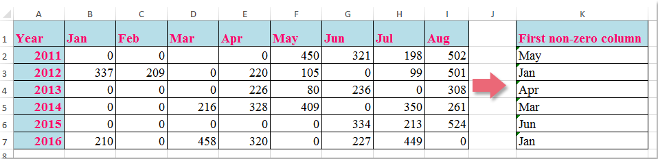
Ենթադրելով, որ դուք ունեք տվյալների մի շարք, այժմ ուզում եք վերադարձնել սյունակի վերնագիրն այդ շարքում, որտեղ տեղի է ունենում առաջին ոչ զրոյական արժեքը, ինչպես ցույց է տրված հետևյալ նկարը. Excel- ում:

փաստաթղթի որոնում առաջին ոչ զրոյական 1

Փնտրեք առաջին ոչ զրոյական արժեքը և վերադարձեք համապատասխան սյունակի վերնագիրը բանաձևով


նետ կապույտ աջ պղպջակ Փնտրեք առաջին ոչ զրոյական արժեքը և վերադարձեք համապատասխան սյունակի վերնագիրը բանաձևով

Անընդմեջ առաջին ոչ զրոյական արժեքի սյունակի վերնագիրը վերադարձնելու համար հետևյալ բանաձևը կարող է օգնել ձեզ, խնդրում ենք արեք հետևյալ կերպ.

Մուտքագրեք այս բանաձևը. =INDEX($B$1:$I$1,MATCH(TRUE,INDEX(B2:I2<>0,),0)) դատարկ բջիջի մեջ, որտեղ ցանկանում եք գտնել արդյունքը, K2, օրինակ, և այնուհետև լրացնելու բռնակը ներքև քաշեք դեպի այն բջիջները, որոնք ցանկանում եք կիրառել այս բանաձևը, և ​​առաջին ոչ զրոյական արժեքի բոլոր համապատասխան սյունակների վերնագրերը վերադարձվում են, ինչպես ցույց է տրված հետևյալ նկարը.

փաստաթղթի որոնում առաջին ոչ զրոյական 2

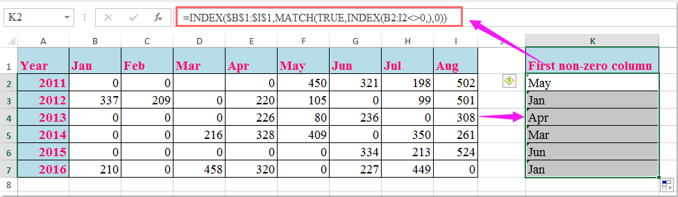
ՆշումՎերոհիշյալ բանաձևում B1: I1 սյունակի վերնագրերն են, որոնք ցանկանում եք վերադարձնել, B2: I2 տողի տվյալներն են, որոնք ցանկանում եք որոնել առաջին ոչ զրոյական արժեքը:

Գրասենյակի արտադրողականության լավագույն գործիքները

🤖 Kutools AI օգնականՀեղափոխություն կատարել տվյալների վերլուծության հիման վրա՝ Խելացի կատարում   |  Ստեղծեք ծածկագիր  |  Ստեղծեք հատուկ բանաձևեր  |  Վերլուծել տվյալները և ստեղծել գծապատկերներ  |  Invoke Kutools-ի գործառույթները...
Հանրաճանաչ հատկություններ: Գտեք, ընդգծեք կամ նույնականացրեք կրկնօրինակները   |  Deleteնջել դատարկ շարքերը   |  Միավորել սյունակները կամ բջիջները՝ առանց տվյալների կորստի   |   Կլոր առանց բանաձևի ...
Super Փնտրել: Բազմաթիվ չափանիշների VLookup    Բազմակի արժեք VLookup  |   VLookup բազմաթիվ թերթերում   |   Fuzzy Փնտրել ....
Ընդլայնված բացվող ցուցակ: Արագ ստեղծեք բացվող ցուցակը   |  Կախված բացվող ցուցակ   |  Բազմակի ընտրություն Drop Down ցուցակ ....
Սյունակի կառավարիչ: Ավելացրեք որոշակի քանակությամբ սյունակներ  |  Տեղափոխել սյունակները  |  Փոխարկել թաքնված սյունակների տեսանելիության կարգավիճակը  |  Համեմատեք միջակայքերը և սյունակները ...
Առանձնահատկություններ: Ցանցի կենտրոնացում   |  Դիզայնի տեսք   |   Մեծ Formula Bar    Աշխատանքային գրքույկի և թերթիկների կառավարիչ   |  Ռեսուրսների գրադարան (Ավտոմատ տեքստ)   |  Ամսաթիվ ընտրող   |  Միավորել աշխատանքային թերթերը   |  Գաղտնագրել/գաղտնազերծել բջիջները    Ուղարկեք նամակներ ըստ ցանկի   |  Սուպեր զտիչ   |   Հատուկ զտիչ (զտել թավ/շեղ/շեղված...) ...
Լավագույն 15 գործիքների հավաքածու12 Տեքստ Գործիքներ (Ավելացրեք տեքստ, Հեռացնել նիշերը, ...)   |   50+ Աղյուսակ Տեսակներ (Գանտի աղյուսակը, ...)   |   40+ Գործնական Բանաձեւեր (Հաշվարկել տարիքը ՝ ելնելով ծննդյան տարեդարձից, ...)   |   19 միացում Գործիքներ (Տեղադրեք QR կոդ, Տեղադրեք նկար ուղուց, ...)   |   12 Փոխարկում Գործիքներ (Բառեր համարներ, Արտարժույթի փոխակերպումը, ...)   |   7 Միաձուլում և պառակտում Գործիքներ (Ընդլայնված կոմբինատ տողեր, Պառակտված բջիջներ, ...)   |   ... եւ ավելին

Լրացրեք ձեր Excel-ի հմտությունները Kutools-ի հետ Excel-ի համար և փորձեք արդյունավետությունը, ինչպես երբեք: Kutools-ը Excel-ի համար առաջարկում է ավելի քան 300 առաջադեմ առանձնահատկություններ՝ արտադրողականությունը բարձրացնելու և ժամանակ խնայելու համար:  Սեղմեք այստեղ՝ Ձեզ ամենաշատ անհրաժեշտ հատկանիշը ստանալու համար...

Նկարագրություն


Office Tab- ը Tabbed ինտերֆեյսը բերում է Office, և ձեր աշխատանքը շատ ավելի դյուրին դարձրեք

  • Միացնել ներդիրներով խմբագրումը և ընթերցումը Word, Excel, PowerPoint- ով, Հրատարակիչ, Access, Visio և Project:
  • Բացեք և ստեղծեք բազմաթիվ փաստաթղթեր նույն պատուհանի նոր ներդիրներում, այլ ոչ թե նոր պատուհաններում:
  • Բարձրացնում է ձեր արտադրողականությունը 50%-ով և նվազեցնում մկնիկի հարյուրավոր սեղմումները ձեզ համար ամեն օր:
Comments (15)
No ratings yet. Be the first to rate!
This comment was minimized by the moderator on the site
Hello, my problem is: a have value 1,2,3,4,...50 that are the number of month. How to denormalize month into real datum. Thank you in advance a lot!!!
This comment was minimized by the moderator on the site
Does anyone know what you would do if your cell that contains a zero has a formula in it? When I use this formula, I end up with whatever the first column header is regardless of whether it is zero or not.
This comment was minimized by the moderator on the site
E como faço pra procurar o primeiro valor diferente de zero da esquerda pra direita?
This comment was minimized by the moderator on the site
Hello, Matheus
If you want to return the first non-zero value from a row, please apply the below formula:
=INDEX(B2:F2,MATCH(TRUE,INDEX(B2:F2<>0,),0))
Please have a try, hope it can help you!
This comment was minimized by the moderator on the site
What if you needed the last non-zero value in an array?

P.S. This was really helpful, thank you so much!
This comment was minimized by the moderator on the site
Hello, Ali,
To get the column header based on the last non-zero value, please apply the below formula, see screenshot:
=INDEX($B$1:$H$1,MAX((COLUMN(B2:H2)-MIN(COLUMN(B2:H2))+1)*(B2:H2<>0)))
Please remember to press Ctrl+Shift+Enter key together.
https://www.extendoffice.com/images/stories/comments/comment-skyyang/doc-last-non-zero.png
Please try, hope it can help you!
This comment was minimized by the moderator on the site
The formula is super helpful and helped me sorted out the situation! Thanks!!! Is there any chance you may please help to also explain how it works?
This comment was minimized by the moderator on the site
How do you look up for the second,third and fourth non-zero value?
This comment was minimized by the moderator on the site
Hello, Robert,
To lookup the second, third or fourth non-zero values and return their columns, please apply the below formula: (After pasting the formula, please press Ctr + Shift + Enter keys together.)
=INDEX($B$1:$I$1,SMALL(IF(B2:I2<>0, COLUMN(B2:I2)-COLUMN(A2)),2))


Note: To extract the third or fourth result, you just need to change the number 2 to 3,4 as you need.

Please have a try, hope it can help you!
This comment was minimized by the moderator on the site
CAN U EXPLIAN HOW THIS FORMULA WORKS
This comment was minimized by the moderator on the site
Hello Priya,I am glad to help. I will separate the formula = INDEX($B$1:$I$1,MATCH(TRUE,INDEX(B2:I2<>0,),0)) into 3 parts, and explain the formula to you step by step.
First, let us see the inner-most formula =INDEX(B2:I2<>0,). This formula returns an array of TRUE and FALSE whether the values of range B2:I2 are equal to 0. Please see the screenshot 1, formula =INDEX(B2:I2<>0,) returns {FALSE,FALSE,FALSE,FALSE,TRUE,TRUE,TRUE,TRUE}.
Second, =MATCH(TRUE,INDEX(B2:I2<>0,),0) =MATCH(TRUE, {FALSE,FALSE,FALSE,FALSE,TRUE,TRUE,TRUE,TRUE}, 0). It returns the position of the first value "TRUE", while 0 in the formula means an exact match. We can see that the first value "TRUE" occurs at the 5th position of the array. Then the second formula returns 5. See the screenshot 2.
Finally,  =INDEX(B1:I1,MATCH(TRUE,INDEX(B2:I2<>0,),0))=INDEX(B1:I1,5). It returns the 5th value of the array B1:I1. We can see in the screenshot that the value is "May". So the final formula returns "May". 
PS: To drag the fill handle down the formula to get the rest of the results, we must make the range B1:I1 absolute. So we add $ to range B1:I1 to keep it absolute. 
Hope my explanation can solve your puzzle. Have a nice day.
Sincerely,Mandy
This comment was minimized by the moderator on the site
Thank you Mandy for illustrating it in detail.
Kindly guide how to get the last non zero value from same formula instead of first non zero value.
Will Match work for that or not?
This comment was minimized by the moderator on the site
Hi MandyZhou,

Thank you for the explanation!
I have a follow-up question.
How would the formula change if you had to look up the year too?
So in the above example, let's assume that column J is 'Year' and that in cell J2 is written '2015'.
And in cell K2 I would need the column header for the first non-zero value of the year in L2 (year 2015, so I would need to find 'Jun' in cell K2).

Thanks in advance for your help!
Jason
This comment was minimized by the moderator on the site
How can I return the second and third, etc non zero value? Your formula is amazing but I am trying to search more keywords from a text so sometimes they are 2 or 3 in the same sentence
This comment was minimized by the moderator on the site
se volessi "l'ultimo" Valore Diverso Da Zero E Restituire L'intestazione Della Colonna Corrispondente Con La Formula?
There are no comments posted here yet
Please leave your comments in English
Posting as Guest
×
Rate this post:
0   Characters
Suggested Locations