Բաց թողնել հիմնական բովանդակությունը

Ինչպե՞ս վերադարձնել Excel- ի մեկ կամ մի քանի չափանիշների հիման վրա մի քանի համընկնող արժեքներ:

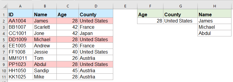
Սովորաբար, որոնեք որոշակի արժեք և վերադարձեք համապատասխան նյութը մեզանից շատերի համար հեշտ է ՝ օգտագործելով VLOOKUP գործառույթը: Բայց երբևէ փորձե՞լ եք վերադարձնել համընկնող բազմաթիվ արժեքներ մեկ կամ մի քանի չափանիշների հիման վրա, ինչպես ցույց է տրված հետևյալ նկարը: Այս հոդվածում ես կներկայացնեմ Excel- ում այս բարդ խնդիրը լուծելու որոշ բանաձևեր:

Վերադարձեք համընկնող բազմաթիվ արժեքներ, որոնք հիմնված են մեկ կամ մի քանի չափանիշների, զանգվածի բանաձևերով


Վերադարձեք համընկնող բազմաթիվ արժեքներ, որոնք հիմնված են մեկ կամ մի քանի չափանիշների, զանգվածի բանաձևերով

Օրինակ, ես ուզում եմ արդյունահանել բոլոր անունները, որոնց տարիքը 28 տարեկան է և գալիս են Միացյալ Նահանգներից, խնդրում եմ կիրառել հետևյալ բանաձևը.

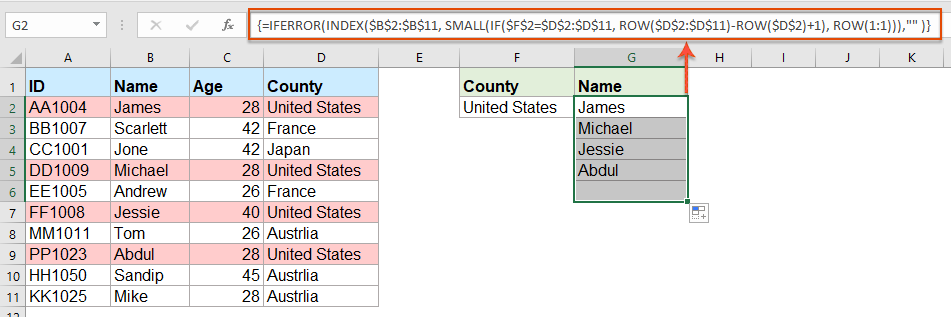
1, Պատճենեք կամ մուտքագրեք ստորև բերված բանաձևը դատարկ բջիջ, որտեղ ցանկանում եք գտնել արդյունքը.

=INDEX($B$2:$B$11, SMALL(IF(COUNTIF($F$2, $C$2:$C$11)*COUNTIF($G$2, $D$2:$D$11), ROW($A$2:$D$11)-MIN(ROW($A$2:$D$11))+1), ROW(A1)), COLUMN(A1))

ՆշումՎերոհիշյալ բանաձևում B2: B11 այն սյունն է, որից վերադարձվում է համապատասխան արժեքը. F2, C2: C11 առաջին պայմանն են և սյունակի տվյալները, որոնք պարունակում են առաջին պայմանը. G2, D2: D11 երկրորդ պայմանն են և սյունակի տվյալները, որոնք պարունակում են այս պայմանը, խնդրում ենք փոխել դրանք ըստ ձեր կարիքի:

2, Հետո, սեղմեք Ctrl + Shift + Մուտք ստեղները `առաջին համապատասխանեցման արդյունքը ստանալու համար, ապա ընտրեք առաջին բանաձևի բջիջը և լրացնելու բռնիչը ներքև քաշեք դեպի բջիջները, մինչև որ ցույց տա սխալի արժեքը:

TipsԵթե ​​պարզապես անհրաժեշտ է վերադարձնել համապատասխանեցման բոլոր արժեքները մեկ պայմանի հիման վրա, խնդրում ենք կիրառել ներքևի զանգվածի բանաձևը.

=IFERROR(INDEX($B$2:$B$11, SMALL(IF($F$2=$D$2:$D$11, ROW($D$2:$D$11)-ROW($D$2)+1), ROW(1:1))),"" )


Ավելի հարաբերական հոդվածներ.

  • Վերադարձեք որոնման մի քանի արժեքներ մեկ ստորակետով առանձնացված բջիջում
  • Excel- ում մենք կարող ենք կիրառել VLOOKUP գործառույթը `աղյուսակի բջիջներից առաջին համապատասխանեցված արժեքը վերադարձնելու համար, բայց, երբեմն, մենք պետք է հանենք բոլոր համապատասխանող արժեքները և այնուհետև առանձնացնենք որոշակի սահմանազատիչով, ինչպիսիք են ստորակետը, գծանշումը և այլն: բջիջը, ինչպես ցույց է տրված հետևյալ նկարը Ինչպե՞ս կարող ենք գտնել և վերադարձնել որոնման բազմաթիվ արժեքներ Excel- ում մեկ ստորակետով առանձնացված բջիջում:
  • Vlookup և միանգամից մի քանի համապատասխան արժեքներ վերադարձնել Google թերթիկում
  • Google թերթի նորմալ Vlookup գործառույթը կարող է օգնել ձեզ գտնել և վերադարձնել տրված տվյալների հիման վրա առաջին համապատասխանող արժեքը: Բայց երբեմն կարող է անհրաժեշտ լինել vlookup և վերադարձնել բոլոր համապատասխանող արժեքները, ինչպես ցույց է տրված հետևյալ նկարը: Google- ի թերթիկում ունե՞ք այս խնդիրը լուծելու լավ և հեշտ եղանակներ:
  • Vlookup և վերադարձնել մի քանի արժեքներ իջնող ցուցակից
  • Excel- ում ինչպե՞ս կարող եք դիտել և վերադարձնել մի քանի համապատասխան արժեքներ բացվող ցուցակից, ինչը նշանակում է, որ երբ բացվող ցուցակից ընտրում եք մեկ կետ, դրա բոլոր հարաբերական արժեքները ցուցադրվում են միանգամից, ինչպես ցույց է տրված հետևյալ նկարը: Այս հոդվածը ես փուլ առ փուլ կներկայացնեմ լուծումը:
  • Vlookup և վերադարձնել մի քանի արժեքներ ուղղահայաց Excel- ում
  • Սովորաբար, առաջին համապատասխան արժեքը ստանալու համար կարող եք օգտագործել Vlookup գործառույթը, բայց, երբեմն, ցանկանում եք վերադարձնել բոլոր համապատասխան գրառումները `ելնելով որոշակի չափանիշի: Այս հոդվածում ես կխոսեմ այն ​​մասին, թե ինչպես vlookup- ը վերադառնալ և վերադարձնել բոլոր համապատասխան արժեքները ուղղահայաց, հորիզոնական կամ մեկ մեկ բջիջում:
  • Vlookup- ը և վերադարձը Excel- ի երկու արժեքների միջև համընկնող տվյալների
  • Excel- ում մենք կարող ենք կիրառել նորմալ Vlookup գործառույթ ՝ տվյալ տվյալների հիման վրա համապատասխան արժեք ստանալու համար: Բայց, երբեմն, մենք ուզում ենք vlookup և վերադարձնել համապատասխան արժեքը երկու արժեքների միջև, ինչպես ցույց է տրված հետևյալ նկարը. Ինչպե՞ս կարող եք գործ ունենալ Excel- ի այս խնդրի հետ:


  • Super Formula Bar (հեշտությամբ խմբագրեք տեքստի և բանաձևի բազմաթիվ տողեր); Ընթերցանության դասավորությունը (հեշտությամբ կարդալ և խմբագրել մեծ թվով բջիջներ); Տեղադրել ֆիլտրացված տիրույթում...
  • Միաձուլել բջիջները / տողերը / սյունակները և տվյալների պահում; Պառակտված բջիջների պարունակությունը; Միավորել կրկնօրինակ տողերն ու գումարը / միջինը... Կանխել կրկնօրինակ բջիջները; Համեմատեք միջակայքերը...
  • Ընտրեք Կրկնօրինակ կամ Եզակի Շարքեր; Ընտրեք դատարկ շարքեր (բոլոր բջիջները դատարկ են); Super Find և Fuzzy Find շատ աշխատանքային գրքույկներում; Պատահական ընտրություն ...
  • Actշգրիտ պատճեն Բազմաթիվ բջիջներ ՝ առանց բանաձևի հղումը փոխելու; Ավտոմատ ստեղծեք հղումներ դեպի մի քանի թերթեր; Տեղադրեք փամփուշտներ, Տուփեր և ավելին ...
  • Սիրված և արագ ներդիր բանաձևեր, Ընդգրկույթներ, գծապատկերներ և նկարներ; Ryածկագրել բջիջները գաղտնաբառով; Ստեղծեք փոստային ցուցակ և նամակներ ուղարկել ...
  • Քաղվածք տեքստ, Տեքստ ավելացնել, հեռացնել ըստ դիրքի, Հեռացնել տարածությունը; Ստեղծել և տպել էջային ենթագոտիներ; Փոխարկել բջիջների բովանդակության և մեկնաբանությունների միջև...
  • Սուպեր զտիչ (պահպանել և կիրառել ֆիլտրի սխեմաները այլ թերթերի վրա); Ընդլայնված տեսակավորում ըստ ամիս / շաբաթ / օր, հաճախականություն և ավելին; Հատուկ զտիչ համարձակ, շեղատառով ...
  • Միավորել աշխատանքային տետրերը և աշխատանքային թերթերը; Միավորել աղյուսակները ՝ հիմնված հիմնական սյունակների վրա; Տվյալները բաժանեք մի քանի թերթերի; Խմբաքանակի փոխակերպում xls, xlsx և PDF...
  • Առանցք սեղանի խմբավորում ըստ շաբաթվա համարը, շաբաթվա օրը և ավելին ... Showույց տալ ապակողպված, կողպված բջիջները տարբեր գույներով; Նշեք այն բջիջները, որոնք ունեն բանաձև / անուն...
kte էջանիշը 201905
  • Միացնել ներդիրներով խմբագրումը և ընթերցումը Word, Excel, PowerPoint- ով, Հրատարակիչ, Access, Visio և Project:
  • Բացեք և ստեղծեք բազմաթիվ փաստաթղթեր նույն պատուհանի նոր ներդիրներում, այլ ոչ թե նոր պատուհաններում:
  • Բարձրացնում է ձեր արտադրողականությունը 50%-ով և նվազեցնում մկնիկի հարյուրավոր սեղմումները ձեզ համար ամեն օր:
officetab ներքևում


Comments (25)
No ratings yet. Be the first to rate!
This comment was minimized by the moderator on the site
Hi, if there are duplicate values (e.g. two adams), how do i make sure that it only returns 1 adam and not 2?
This comment was minimized by the moderator on the site
Hello, Bobby,
To extract only unique matching values, you should apply the below formula:
After pasting the formula, please press Ctrl + Shift + Enter keys together to get the correct result.
=IFERROR(INDEX($B$2:$B$5, MATCH(0, COUNTIF(H1:$H$1, $B$2:$B$5)+IF($D$2:$D$5<>$G$2, 1, 0)+IF($C$2:$C$5<>$F$2, 1, 0), 0)), "")

Please have a try, hope it can help you!
This comment was minimized by the moderator on the site
Hi,

Thanks for posting these examples.
I'm trying to implement this in my own sheet, but don't get it to work (maybe because I'm using an europe version of excel)?

I want to get the dates of the days that I had my shifts or that I have worked 'some' (>0) hours for a client.

So in I3 is the name and in J3 the month. K3 and L3 are the shifts (1 is worked) and hours (don't know how to set this, should be more than zero)

My expected results are in:
Shifts: I7 and I8
hours: J7

So I worked more than 0 hours for 'person 2' in oktober on 3-10-2022
had shifts for person 2 on '10-10-2022' and 28-10-2022

When I add '=INDEX($B$2:$B$11, SMALL(IF(COUNTIF($F$2, $C$2:$C$11)*COUNTIF($G$2, $D$2:$D$11), ROW($A$2:$D$11)-MIN(ROW($A$2:$D$11))+1), ROW(A1)), COLUMN(A1))' in my excel sheet, it doesn't allow the comma between the different parts of the formula.
So I need to change them to ';'.
But when I try it it always says: '#NAME?'

So can someone help me with this?

Kind regards,

Bas
[img]https://drive.google.com/file/d/1iIPQKuj_PNhqWyWlwJ4IQTqGNEd6B9Hw/view?usp=share_link[/img]
This comment was minimized by the moderator on the site
Hi,

First, thank you for sharing!

Can you please provide a solution to the case below:

I have 3 columns (A: Containing reference information, B: Containing information to be searched, C: Search result)

Image url is provided below

https://ibb.co/VHCd09K

Column A-------------------------Column B------------Column C
File Name-------------------------Name----------------File Name, Document Name, Element Name, Name
Changed Element-----------------Element--------------Changed Element, Element Name, Element ID
Column Location
Document Name
Element Name
Name
Category
Warranty
Slope
Element ID

What I need is to search in column A for any partial match with cell B2 (Name) or B3 (Element) and get the result in one cell,

Thank you, Behzad
This comment was minimized by the moderator on the site
Hello, Behzad
Maybe the below User Defined Function can help you.
Public Function ConcatPartLookUp(rngInput As Range, rngSource As Range, Optional strDelimiter As String, Optional blCaseSensitive)
Dim rng As Range
If strDelimiter = "" Then strDelimiter = ","
If IsMissing(blCaseSensitive) Then
    blCaseSensitive = False
Else
    blCaseSensitive = True
End If
For Each rng In rngSource
    If blCaseSensitive Then
        If InStr(1, rng.Value, rngInput.Value, vbBinaryCompare) > 0 Then ConcatPartLookUp = ConcatPartLookUp & strDelimiter & rng.Value
    Else
        If InStr(1, rng.Value, rngInput.Value, vbTextCompare) > 0 Then ConcatPartLookUp = ConcatPartLookUp & strDelimiter & rng.Value
    End If
Next
If Len(ConcatPartLookUp) > 0 Then ConcatPartLookUp = Mid(ConcatPartLookUp, 2, Len(ConcatPartLookUp))
End Function


After copying and pasting this code, and then use this formula:=ConcatPartLookUp(B2,$A$2:$A$8) to get the result you need.
Please have a try, hope it can help you!
This comment was minimized by the moderator on the site
Heyi, thank you for the formula. It worked for "fixed" values / text as criterias. However, one of the criterias i'm trying to use is a condition (values <>0 ), but does not work the described formula. Do you guys know what should i change to adapt the formula so I can have a condition as one of the criterias, please?

Best,

João
This comment was minimized by the moderator on the site
Hello, Marcus
To solve your problem, please view this article:
https://www.extendoffice.com/documents/excel/6393-excel-vlookup-function.html#b3-2
There are some detailed explanations of this task. You just need to change the criteira to your own.
Thank you!
This comment was minimized by the moderator on the site
Hi,

if in cell H1 i write "Name" and wanted to link that with the formula, how would that work?
Then I could write "ID" in cell H1 and would automatically get as a result: AA1004; DD1009; PP1023 (for the first formula)

Thank you in advance!
This comment was minimized by the moderator on the site
Hello, Marie
Sorry, i can't get the point of your first problem, could you explain your problem more clearly and detailedly? Or you can insert a screenshot here to describe your problem.
As for the second question, you just need to change the cell reference as this:
=INDEX($A$2:$A$11, SMALL(IF(COUNTIF($F$2, $C$2:$C$11)*COUNTIF($G$2, $D$2:$D$11), ROW($A$2:$D$11)-MIN(ROW($A$2:$D$11))+1), ROW(A1)), COLUMN(A1))

Remeber to press Ctrl + Shift + Enter keys together.
Please try, hope it can help you!
This comment was minimized by the moderator on the site
Hello,
what would be needed to expand the first formula in the following case:
Some IDs are Blank (e.g. cell A5 is blank) and I would like an additional condition outputting lines only when the IDs are not blank. (So the output should then be James and Abdul.
Thanks!
This comment was minimized by the moderator on the site
Hello, Jo,
To solve your problem, please apply the below formula:
=INDEX($B$2:$B$11, SMALL(IF(COUNTIF($F$2, $C$2:$C$11)*COUNTIF($G$2, $D$2:$D$11)*($A$2:$A$11<>0), ROW($A$2:$D$11)-MIN(ROW($A$2:$D$11))+1), ROW(A1)), COLUMN(A1))

Please have a ry, hope it can help you!
This comment was minimized by the moderator on the site
hello,
ive tried using the formula and it either generates a value of 0 or the image attached
This comment was minimized by the moderator on the site
Hello, Milku
Your screenshot showed WPS software of MAC version, so I am not sure whether our formula is available.
I uploaded an Excel file to here, you can try to see if it can calculate correctly in you environment.
Thank you!
This comment was minimized by the moderator on the site
When I use the second formula and drag down, nothing appears. The formula result (fx) says it should be returning something but it is blank. How do I correct this?
This comment was minimized by the moderator on the site
Hello Alysia,

Glad to help. I tried the second formula in the article and drag the formula down, the rest of results were returned. I think there may be two reasons for your problem. First, maybe you forget to press Ctrl + Shift + Enter keys to enter the formula. Second, the matching result is only one, so no other results are not returned. Please have a check.

Sincerely,
Mandy
This comment was minimized by the moderator on the site
Hi,

I was wondering if it at all possible to enter a 2nd criteria but from the same range as the 1st criteria,

For example with the used example above i would like to search for the names of people from both America and France So cell F3 would have France, Scarlett & Andrew would also populate in the list in Column G

Thank you for assistance in advance.
This comment was minimized by the moderator on the site
Hello Nick,

Glad to help. If you want to get the names of people from both America and France, I advise you to use our formula twice to get the result. Please see the screenshot, In F2 and G2 are values "United States" and "France". Apply formula =IFERROR(INDEX($B$2:$B$11, SMALL(IF($F$2=$D$2:$D$11, ROW($D$2:$D$11)-ROW($D$2)+1), ROW(1:1))),"" ) to get the results for America. And apply formula =IFERROR(INDEX($B$2:$B$11, SMALL(IF($G$2=$D$2:$D$11, ROW($D$2:$D$11)-ROW($D$2)+1), ROW(1:1))),"" ) to get the results for France. It's simple. Please have a try.

Sincerely,
Mandy
This comment was minimized by the moderator on the site
In the first example, what change to the formula would be needed to return everyone who was less than 28 years old?
There are no comments posted here yet
Load More
Please leave your comments in English
Posting as Guest
×
Rate this post:
0   Characters
Suggested Locations