Բաց թողնել հիմնական բովանդակությունը

Ինչպե՞ս արժեք գտնել Excel- ում ստորակետերով առանձնացված բջիջում:

Ենթադրելով, որ դուք ունեք սյուն, պարունակում է ստորակետերով առանձնացված արժեքներ, ինչպիսիք են Sales, 123, AAA, և այժմ ուզում եք պարզել, թե արդյոք 123 արժեքը ստորակետով առանձնացված բջիջում, ինչպե՞ս կարող եք դա անել: Այս հոդվածը կներկայացնի խնդիրը լուծելու մեթոդ:

Գտեք արժեքը բանաձևով ստորակետերով առանձնացված բջիջում


Գտեք արժեքը բանաձևով ստորակետերով առանձնացված բջիջում

Հետևյալ բանաձևը կարող է օգնել Excel- ում ստորակետերով առանձնացված բջիջում արժեք գտնել: Խնդրում եմ արեք հետևյալ կերպ.

1. Ընտրեք դատարկ բջիջ, մուտքագրեք բանաձև =IF(ISNUMBER(SEARCH(123,A2)),"yes","no") մուտքագրեք Formula Bar և սեղմեք Enter ստեղնը: Տեսեք,

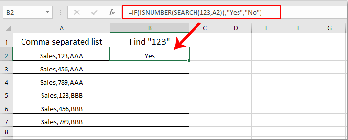
Նշում: բանաձևում A2- ն այն բջիջն է, որը պարունակում է ստորակետերով առանձնացված արժեքներ:

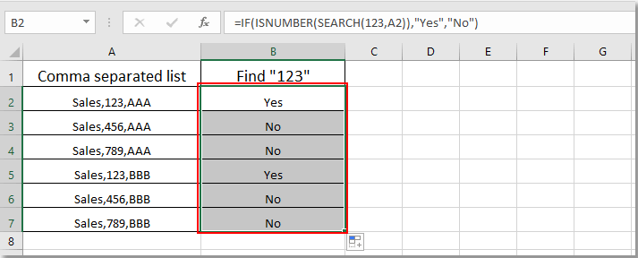
2. Շարունակեք ընտրել արդյունքի բջիջը և ներքև քաշել Լրացնելու բռնակը `բոլոր արդյունքները ստանալու համար: Եթե ​​«123» արժեքը ստորակետերով առանձնացված բջիջներում է, ապա արդյունքը կստանաք որպես «Այո»; հակառակ դեպքում արդյունքը կստանաք որպես «Ոչ»: Տեսեք,


Առնչվող հոդվածներ քանակը:

Գրասենյակի արտադրողականության լավագույն գործիքները

🤖 Kutools AI օգնականՀեղափոխություն կատարել տվյալների վերլուծության հիման վրա՝ Խելացի կատարում   |  Ստեղծեք ծածկագիր  |  Ստեղծեք հատուկ բանաձևեր  |  Վերլուծել տվյալները և ստեղծել գծապատկերներ  |  Invoke Kutools-ի գործառույթները...
Հանրաճանաչ հատկություններ: Գտեք, ընդգծեք կամ նույնականացրեք կրկնօրինակները   |  Deleteնջել դատարկ շարքերը   |  Միավորել սյունակները կամ բջիջները՝ առանց տվյալների կորստի   |   Կլոր առանց բանաձևի ...
Super Փնտրել: Բազմաթիվ չափանիշների VLookup    Բազմակի արժեք VLookup  |   VLookup բազմաթիվ թերթերում   |   Fuzzy Փնտրել ....
Ընդլայնված բացվող ցուցակ: Արագ ստեղծեք բացվող ցուցակը   |  Կախված բացվող ցուցակ   |  Բազմակի ընտրություն Drop Down ցուցակ ....
Սյունակի կառավարիչ: Ավելացրեք որոշակի քանակությամբ սյունակներ  |  Տեղափոխել սյունակները  |  Փոխարկել թաքնված սյունակների տեսանելիության կարգավիճակը  |  Համեմատեք միջակայքերը և սյունակները ...
Առանձնահատկություններ: Ցանցի կենտրոնացում   |  Դիզայնի տեսք   |   Մեծ Formula Bar    Աշխատանքային գրքույկի և թերթիկների կառավարիչ   |  Ռեսուրսների գրադարան (Ավտոմատ տեքստ)   |  Ամսաթիվ ընտրող   |  Միավորել աշխատանքային թերթերը   |  Գաղտնագրել/գաղտնազերծել բջիջները    Ուղարկեք նամակներ ըստ ցանկի   |  Սուպեր զտիչ   |   Հատուկ զտիչ (զտել թավ/շեղ/շեղված...) ...
Լավագույն 15 գործիքների հավաքածու12 Տեքստ Գործիքներ (Ավելացրեք տեքստ, Հեռացնել նիշերը, ...)   |   50+ Աղյուսակ Տեսակներ (Գանտի աղյուսակը, ...)   |   40+ Գործնական Բանաձեւեր (Հաշվարկել տարիքը ՝ ելնելով ծննդյան տարեդարձից, ...)   |   19 միացում Գործիքներ (Տեղադրեք QR կոդ, Տեղադրեք նկար ուղուց, ...)   |   12 Փոխարկում Գործիքներ (Բառեր համարներ, Արտարժույթի փոխակերպումը, ...)   |   7 Միաձուլում և պառակտում Գործիքներ (Ընդլայնված կոմբինատ տողեր, Պառակտված բջիջներ, ...)   |   ... եւ ավելին

Լրացրեք ձեր Excel-ի հմտությունները Kutools-ի հետ Excel-ի համար և փորձեք արդյունավետությունը, ինչպես երբեք: Kutools-ը Excel-ի համար առաջարկում է ավելի քան 300 առաջադեմ առանձնահատկություններ՝ արտադրողականությունը բարձրացնելու և ժամանակ խնայելու համար:  Սեղմեք այստեղ՝ Ձեզ ամենաշատ անհրաժեշտ հատկանիշը ստանալու համար...

Նկարագրություն


Office Tab- ը Tabbed ինտերֆեյսը բերում է Office, և ձեր աշխատանքը շատ ավելի դյուրին դարձրեք

  • Միացնել ներդիրներով խմբագրումը և ընթերցումը Word, Excel, PowerPoint- ով, Հրատարակիչ, Access, Visio և Project:
  • Բացեք և ստեղծեք բազմաթիվ փաստաթղթեր նույն պատուհանի նոր ներդիրներում, այլ ոչ թե նոր պատուհաններում:
  • Բարձրացնում է ձեր արտադրողականությունը 50%-ով և նվազեցնում մկնիկի հարյուրավոր սեղմումները ձեզ համար ամեն օր:
Comments (17)
No ratings yet. Be the first to rate!
This comment was minimized by the moderator on the site
It’s working for single value, how do I find multiple values. Example: search values (101, 402,110) it might have all 3 or only one or two values and find cell will have any of three or all three or two.
Scenarios
1. Cell 1: 101 cell 2: 101,402,110,202,220
2. Cell 1: 101,402 cell 2: 101,402,202,220,110
3. Cell 1: 110,101,402 cell 2: 101,402,202,220,110

Pls advice
This comment was minimized by the moderator on the site
Hey, I still cant figure this out. I am still having the same problem. instead of using number in the formula I am using a cell reference. for example if i am searching for "1"(Q$1) in (123, 25,29,200)($J2) it is still giving me YES. The formula is =IF(ISNUMBER(SEARCH(Q$1,$J2)),"yes","no")

PS: I have a big data set I cannot put commas before and after in every cell. Will appreciate a solution
This comment was minimized by the moderator on the site
Hi Hassam

Just use the following formula without the IF function. If the number matches exactly, you will get the result "TRUE", otherwise you will get the result "FALSE".
=ISNUMBER(FIND(",1,",","&$J2&","))
https://www.extendoffice.com/images/stories/comments/comment-picture-zxm/match.png
This comment was minimized by the moderator on the site
Hi All, I have a cell that has multiple countries separated by commas
Example : A2 cell value is (India, Japan, Malaysia, Greater China)
Column G has the country names
Now , I need to find look for a formula that compares value from column G to value in A2 cell .
If the value matches, then return true otherwise return False
This comment was minimized by the moderator on the site
Hi Mohini Verma,
The formula can be modified as follows:
=IF(ISNUMBER(SEARCH(G2,A2)),"TRUE","FALSE")
This comment was minimized by the moderator on the site
How about this please, I need to get the values in A and equate them with the figures in C and return the values in B separated as in commas respectively to C.

Thanks
This comment was minimized by the moderator on the site
Hi duncan,
If you are using Excel for 365, the following formula can help solving the problem.
=TEXTJOIN(",",TRUE,XLOOKUP(TRANSPOSE(VALUE(TEXTSPLIT(D1,","))),A1:A3,B1:B3,"",0,1))
This formula only works in Excel for 365. For other Excel versions other than Excel for 365, I have not found a formula that handles it..
https://www.extendoffice.com/images/stories/comments/comment-picture-zxm/find-value.png
This comment was minimized by the moderator on the site
Hi Please help

I have table in Excel with two columns A & B, under A there are value Eg A2 Cell has 1,2,2,1,2,1,2 etc ( only has two numbers 1 and 2 but needs to recognise it has only 1 & 2 in the whole cell and no other number) and A3 has 1,1,1 and A4 has 0, A5 has 2,2,2,2 and A6 has 20. i want B2 should return the value for A2 as Asia, B3 Africa, B4 as None, B5 as America and B6 as Europe. I thought i could use the if formula but it is not able to recognise comma separated numbers and return value). Please Help
This comment was minimized by the moderator on the site
Hello!
This is a really cool formula, but it has ... flaw? ... that I cannot figure out how to work around it. "Flaw" is not the correct word, but I cannot think (it's 8:30 am on Monday) of the right word.
When you are looking for any part of a number, you get "yes". So, the following all return "yes":
=IF(ISNUMBER(SEARCH(12,A2)),"yes","no")
=IF(ISNUMBER(SEARCH(23,A2)),"yes","no")
=IF(ISNUMBER(SEARCH(3,A2)),"yes","no")

I tried wrapping the numbers in quotes to no avail. The formula works perfectly for the example's use case, in which all of the numbers are of the same length. But if you are looking for a shorter number that happens to appear in the string, you get a false positive.
Is there an alternative to "SEARCH" that is more literal (again, is that the word? haha)? 
Thanks! 
This comment was minimized by the moderator on the site
Hi Scott S.,Do you mean search for the exact string?
This comment was minimized by the moderator on the site
Hi, Crystal.
Yes, I suppose that is the way to phrase it. 
The current solution will return “Yes” for any part of the number string. So the numbers 1, 2, 3, 12, 23, and 123 will all return “Yes”. 
I have been trying to come up with a solution that will search a string of numbers and return “Yes” for an exact match. 
This comment was minimized by the moderator on the site
Hi Scott S,Thanks for your feedback. I haven't found the solution yet and will get back to you if I found it.
This comment was minimized by the moderator on the site
I have found a solution. If you add a comma to the left and right of your list it will require the search function to find an exact match from comma to comma. See example below:
=IF(ISNUMBER(SEARCH(",12,",A2)),"yes","no")

,312,123,10,112,126,
This will return false because there is no variable from comma to comma (,12,) that matches the search. 
If you need further clarification let me know and ill post a better example.I was having the same problem when automating a report for my boss and had an epiphany. :)
This comment was minimized by the moderator on the site
Hey, I still cant figure this out. I am still having the same problem. instead of using number in the formula I am using a cell reference. for example if i am searching for "1"(Q$1) in (123, 25,29,200)($J2) it is still giving me YES. The formula is =IF(ISNUMBER(SEARCH(Q$1,$J2)),"yes","no")

PS: I have a big data set I cannot put commas before and after in every cell. Will appreciate a solution
This comment was minimized by the moderator on the site
I have found a solution for this. If you add a comma to the left and right of your list and include them (like a sandwich) in your search it'll allow you to find an exact match. Example below:
,123,231,321,122,321,1,2,3,23,
SEARCH(",23,")
This way it forces the search to match from one comma to the other rather than just part of the entry from the list. Hope this is what you were looking for?
This comment was minimized by the moderator on the site
Good Morning to all.I have a excel question that how to count comma separated specific values in a single cell in excel.I want to count no of 15's in a single cell that contains 15,215,15,155,45,1515,15 I need the result 3. Is there any formula in excel.
This comment was minimized by the moderator on the site
Yes, there is a function in Excel that can do this for you. However, as explained in the problem above to gain better accuracy for your data add a comma to the left and right of your list and include it in your search. See example below:
,15,215,15,155,45,1515,15,
=COUNTIF(A1, ",15,")
The explanation of this formula is as follows: =COUNTIF(cell number or range, value your looking for/counting)
Let me know if you need a better example.
There are no comments posted here yet
Please leave your comments in English
Posting as Guest
×
Rate this post:
0   Characters
Suggested Locations