Creating a search box in Excel enhances the functionality of your spreadsheets by making it easier to filter and access specific data quickly. This guide covers several methods to implement a search box, catering to different versions of Excel. Whether you're a beginner or an advanced user, these steps will help you set up a dynamic search box using features like the FILTER function, Conditional Formatting, and various formulas.

• Easily create a search box with the FILTER ֆունկցիան
  (available in Excel 2019 and later, Excel for Microsoft 365)
• Create a search box using Պայմանական ֆորմատավորում
  (available in all Excel versions)
• Create a search box with formula combinations
  (available in all Excel versions)

Easily create a search box with the FILTER function

• This function automatically updates the output as your data changes.
• The FILTER function can return any number of results, from a single row to thousands, depending on how many entries in your dataset match the criteria you've set.

Here I will show you how to use the FILTER function to create a search box in Excel.

Step 1: Insert a text box and configure properties

1. Կարդացեք Երեվակիչ էջանշանը, սեղմեք Տեղադրել > Տext Box (ActiveX Control).
   Ակնարկ: Եթե Երեվակիչ tab is not shown on the ribbon, you can enable it by following the instructions on this tutorial: Ինչպե՞ս ցուցադրել / ցուցադրել մշակողի ներդիրը Excel ժապավենում:
   
2. The cursor will turn into a cross, and then you need to drag the cursor to draw the text box at the location in the worksheet where you want to place the text box. After drawing the text box, release the mouse.
   
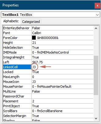
3. Right click the text box and select Հատկություններ համատեքստի ընտրացանկից:
   
4. Է Հատկություններ pane, link the text box to a cell by entering the cell reference in the LinkedCell- ը field. For example, typing "J2" ensures that any data entered in the text box automatically updates in cell J2, and vice versa.
   
5. Սեղմեք է Դիզայնի ռեժիմ տակ Երեվակիչ tab to exit the Design Mode.
   

The text box now allows you to enter text.

Step 2: Apply the FILTER function

1. Before using the FILTER function, copy the original header row to a new area. Here I place the header row under the search box.
   Ակնարկ: This approach allows users to clearly see the results under the same column headings as the original data.
   
2. Select the cell under the first header (e.g. I5 in this example), enter the following formula into it and press the Մտնել արդյունքը ստանալու բանալին:

   =FILTER(Sheet2!$A$5:$G$281,Sheet2!$B$5:$B$281=J2,"No data found")

   
   As shown in the above screenshot, since the text box now has no input, the formula displays the result "Տվյալներ չեն գտնվել» I5.

Result: Test the search box

Let's now test the search box. In this example, when I enter a customer's name in the search box, the corresponding results will be filtered and displayed immediately.

Create a search box using Conditional Formatting

Conditional Formatting can be used to highlight data that matches a search term, indirectly creating a search box effect. This method does not filter out data but visually guides you to the relevant cells. This section will show you how to create a search box using Conditional Formatting in Excel.

Step 1: Insert a text box and configure properties

1. Կարդացեք Երեվակիչ էջանշանը, սեղմեք Տեղադրել > Տext Box (ActiveX Control).
   Ակնարկ: Եթե Երեվակիչ tab is not shown on the ribbon, you can enable it by following the instructions on this tutorial: Ինչպե՞ս ցուցադրել / ցուցադրել մշակողի ներդիրը Excel ժապավենում:
   
2. The cursor will turn into a cross, and then you need to drag the cursor to draw the text box at the location in the worksheet where you want to place the text box. After drawing the text box, release the mouse.
   
3. Right click the text box and select Հատկություններ համատեքստի ընտրացանկից:
   
4. Է Հատկություններ pane, link the text box to a cell by entering the cell reference in the LinkedCell- ը field. For example, typing "J3" ensures that any data entered in the text box automatically updates in cell J3, and vice versa.
   
5. Սեղմեք է Դիզայնի ռեժիմ տակ Երեվակիչ tab to exit the Design Mode.
   

The text box now allows you to enter text.

Step 2: Apply the Conditional Formatting for searching data

1. Select the entire data range to be searched. Here I select the range A3:G279.
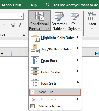
2. Տակ է Գլխավոր էջանշանը, սեղմեք Պայմանական ֆորմատավորում > Նոր կանոն.
   
3. Է Ձևաչափման նոր կանոն երկխոսության տուփ:
   1. ընտրել Օգտագործեք բանաձև `որոշելու համար, թե որ բջիջները ձևափոխել է Ընտրեք կանոնի տեսակը տարբերակները.
   2. Enter the following formula into the Ձևաչափեք արժեքները, երբ այս բանաձեւը ճիշտ է տուփ:

      =$B3=$J$3

      Այստեղ, $ B3 represents the first cell in the column you want to match with the search criteria in the selected range, and $ J $ 3 is the cell linked to the search box.
   3. Սեղմեք է Ֆորմատ button to specify a fill color for the search results.
   4. Սեղմեք է OK կոճակ Տեսեք,
      

Արդյունք

Let’s now test the search box. In this example, when I enter a customer’s name into the search box, the corresponding rows that contain this customer in column B will be immediately highlighted with the specified fill color.

Create a search box with formula combinations

If you are not using the latest version of Excel and prefer not to only highlight rows, the method described in this section may be helpful. You can use a combination of Excel formulas to create a functional search box in any version of Excel. Please follow the steps below.

Step 1: Create a list of unique values from the search column

1. In this case, I select and copy the range B4: B281 to a new worksheet.
2. After pasting the range in a new worksheet, keep the pasted data selected, go to the Ամսաթիվ ներդիր եւ ընտրեք Հեռացնել կրկնօրինակները.
   
3. Բացման մեջ Հեռացնել կրկնօրինակները երկխոսության տուփ, կտտացրեք OK կոճակը:
   
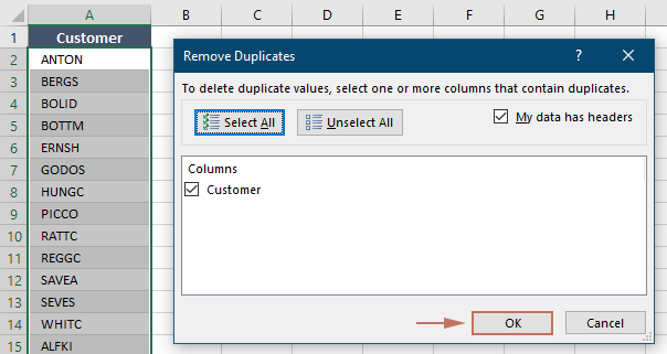
4. A Microsoft Excel- ը prompt box then pops up to show how many duplicates are removed. Click OK.
   
5. After removing duplicates, select all the unique values in the list, excluding the header, and assign a name to this range by entering it in the Անուն box. Here I named the range as Հաճախորդ.
   

Step 2: Insert a combo box and configure properties

1. Go back to the worksheet containing the data set you want to search. Go to the Երեվակիչ էջանշանը, սեղմեք Տեղադրել > Combo Box (ActiveX հսկողություն).
   Ակնարկ: Եթե Երեվակիչ tab is not shown on the ribbon, you can enable it by following the instructions on this tutorial: Ինչպե՞ս ցուցադրել / ցուցադրել մշակողի ներդիրը Excel ժապավենում:
   
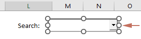
2. The cursor will turn into a cross, and then you need to drag the cursor to draw the combo box at the location in the worksheet where you want to place the search box. After drawing the combo box, release the mouse.
   
3. Right click the combo box and select Հատկություններ համատեքստի ընտրացանկից:
   
4. Է Հատկություններ պատուհան:
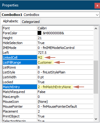
   1. Link the combo box to a cell by entering the cell reference in the LinkedCell- ը field. Her I type "M2".
      Tip: Specify this field ensures that any data entered in the combo box will automatically update in cell M2, and vice versa.
   2. Է ListFillRange դաշտ, մուտքագրեք range name you specified for the unique list in Step 1.
   3. Փոխեք MatchEntry դաշտը 2 – fmMatchEntryNone.
   4. Փակեք Հատկություններ հաց.
      
5. Սեղմեք է Դիզայնի ռեժիմ տակ Երեվակիչ tab to exit the Design Mode.
   

You can now select any item from the combo box or type in the text to search for.

Step 3: Apply formulas

1. Create three helper columns adjacent to the original data range. See screenshot:
   
2. In the cell (H5) under heading of the first helper column, enter the following formula and press Մտնել.

   =ROWS($B$5:B5)

   Այստեղ B5 is the cell containing the first custmer's name of the column to be searched.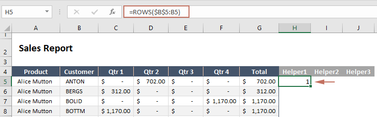
   
3. Double click the lower right corner of the formula cell, the following cell will automatically fill in the same formula.
   
4. In the cell (I5) under the second helper column header, enter the following formula and press Մտնել. And then double click the lower right corner of the formula cell to automatically fill the cells below with the same formula.

   =IF(ISNUMBER(SEARCH($M$2,B5)),H5,"")

   Այստեղ M2 բջիջն է, որը կապված է համակցված տուփի հետ:
   
5. In the cell (J5) under the third helper column header, enter the following formula and press Մտնել. And then double click the lower right corner of the formula cell to automatically fill the cells below with the same formula.

   =IFERROR(SMALL($I$5:$I$281,H5),"") 

   
6. Copy the original header row to a new area. Here I place the header row under the search box.
   
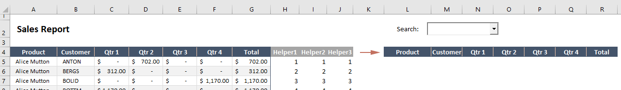
7. Select the cell under the first header (e.g. L5 in this example), enter the following formula into it and press the Enter key.

   =IFERROR(INDEX($A$5:$G$281,$J5,COLUMNS($L$4:L4)),"")

   Այստեղ A5: G281 is the entire data range that you want to displayed in the result cell.
   
8. Select this formula cell, drag the Լրացրեք բռնակ to the right and then down to apply the formula to the corresponding columns and rows.
   
   Notes:

   • Since there is no input in the search box, the results of the formula will show the raw data.
   • This method is case-insensitive, meaning it will match text regardless of whether you type in uppercase or lowercase letters.

Արդյունք

Let's now test the search box. In this example, when I enter or select a customer's name from the combo box, the corresponding rows that contain that customer name in column B will be filtered and immediately displayed in the result range.

Creating a search box in Excel can significantly improve how you interact with your data, making your spreadsheets more dynamic and user-friendly. Whether you choose the simplicity of the FILTER function, the visual assistance of Conditional Formatting, or the versatility of formula combinations, each method provides valuable tools to enhance your data manipulation capabilities. Experiment with these techniques to find which works best for your specific needs and data scenarios. For those eager to delve deeper into Excel's capabilities, our website boasts a wealth of tutorials. Բացահայտեք Excel-ի ավելի շատ խորհուրդներ և հնարքներ այստեղ.

Առնչվող հոդվածներ