Բաց թողնել հիմնական բովանդակությունը

Ինչպե՞ս կողպել նշված բջիջները ՝ առանց Excel- ի ամբողջ աշխատանքային թերթը պաշտպանելու:

Սովորաբար, անհրաժեշտ է պաշտպանել ամբողջ աշխատանքային թերթը ՝ բջիջները խմբագրումից արգելափակելու համար: Կա՞ որևէ մեթոդ `բջիջները կողպելու համար` առանց ամբողջ աշխատանքային թերթը պաշտպանելու: Այս հոդվածը ձեզ համար խորհուրդ է տալիս VBA մեթոդ:

Կողպեք նշված բջիջները ՝ առանց ամբողջ VBA- ով պաշտպանելու աշխատանքային թերթիկը


Կողպեք նշված բջիջները ՝ առանց ամբողջ VBA- ով պաշտպանելու աշխատանքային թերթիկը

Ենթադրելով, որ անհրաժեշտ է կողպել A3 և A5 բջիջները ընթացիկ աշխատանքային թերթում, հետևյալ VBA կոդը կօգնի ձեզ հասնել դրան ՝ առանց ամբողջ աշխատանքային թերթը պաշտպանելու:

1. Աջ կտտացրեք թերթիկի ներդիրին և ընտրեք Դիտել կոդը աջ կտտացնելու ցանկից:

2. Դրանից հետո պատճենեք և կպցրեք ստորև նշված VBA կոդը օրենսգրքի պատուհանում: Տեսեք,

VBA կոդ. Կողպեք նշված բջիջները ՝ առանց ամբողջ աշխատանքային թերթը պաշտպանելու

Private Sub Worksheet_SelectionChange(ByVal Target As Range)
    If Target.Column = 1 Then
        If Target.Row = 3 Or Target.Row = 5 Then
            Beep
            Cells(Target.Row, Target.Column).Offset(0, 1).Select
        End If
    End If
End Sub

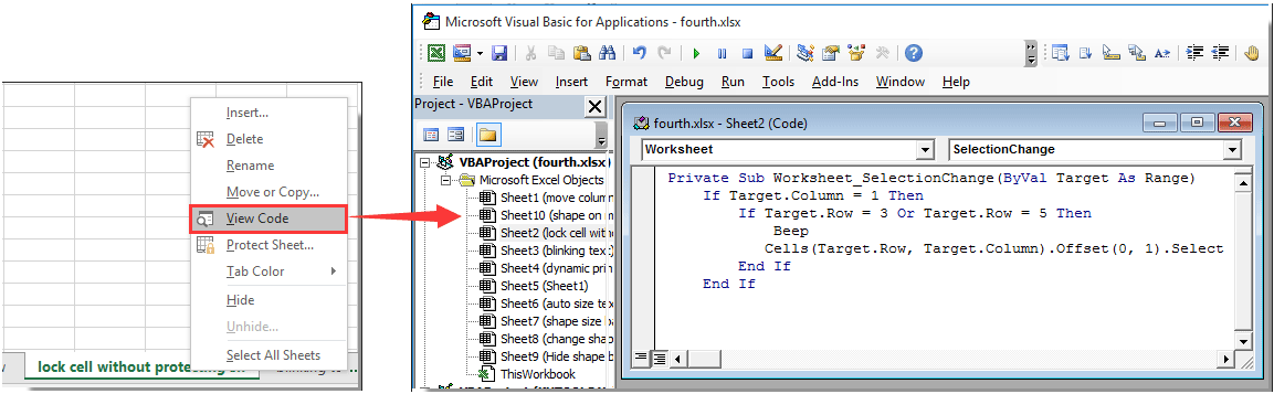
ՆշումԿոդում, Սյունակ 1, Տող = 3 և Տող = 5 նշեք A3 և A5 բջիջները ընթացիկ աշխատաթերթում կփակվեն ծածկագիրը գործարկելուց հետո: Դուք կարող եք փոխել դրանք, ինչպես ձեզ հարկավոր է:

3. Սեղմեք ալտ + Q ստեղները միաժամանակ փակելու համար Microsoft Visual Basic հավելվածների համար պատուհան.

Այժմ A3 և A5 բջիջները կողպված են ընթացիկ աշխատանքային թերթում: Եթե ​​ընթացիկ աշխատաթերթում փորձեք ընտրել A3 կամ A5 բջիջները, կուրսորը ավտոմատ կերպով կտեղափոխվի աջ հարակից բջիջ:


Առնչվող հոդվածներ:

Գրասենյակի արտադրողականության լավագույն գործիքները

🤖 Kutools AI օգնականՀեղափոխություն կատարել տվյալների վերլուծության հիման վրա՝ Խելացի կատարում   |  Ստեղծեք ծածկագիր  |  Ստեղծեք հատուկ բանաձևեր  |  Վերլուծել տվյալները և ստեղծել գծապատկերներ  |  Invoke Kutools-ի գործառույթները...
Հանրաճանաչ հատկություններ: Գտեք, ընդգծեք կամ նույնականացրեք կրկնօրինակները   |  Deleteնջել դատարկ շարքերը   |  Միավորել սյունակները կամ բջիջները՝ առանց տվյալների կորստի   |   Կլոր առանց բանաձևի ...
Super Փնտրել: Բազմաթիվ չափանիշների VLookup    Բազմակի արժեք VLookup  |   VLookup բազմաթիվ թերթերում   |   Fuzzy Փնտրել ....
Ընդլայնված բացվող ցուցակ: Արագ ստեղծեք բացվող ցուցակը   |  Կախված բացվող ցուցակ   |  Բազմակի ընտրություն Drop Down ցուցակ ....
Սյունակի կառավարիչ: Ավելացրեք որոշակի քանակությամբ սյունակներ  |  Տեղափոխել սյունակները  |  Փոխարկել թաքնված սյունակների տեսանելիության կարգավիճակը  |  Համեմատեք միջակայքերը և սյունակները ...
Առանձնահատկություններ: Ցանցի կենտրոնացում   |  Դիզայնի տեսք   |   Մեծ Formula Bar    Աշխատանքային գրքույկի և թերթիկների կառավարիչ   |  Ռեսուրսների գրադարան (Ավտոմատ տեքստ)   |  Ամսաթիվ ընտրող   |  Միավորել աշխատանքային թերթերը   |  Գաղտնագրել/գաղտնազերծել բջիջները    Ուղարկեք նամակներ ըստ ցանկի   |  Սուպեր զտիչ   |   Հատուկ զտիչ (զտել թավ/շեղ/շեղված...) ...
Լավագույն 15 գործիքների հավաքածու12 Տեքստ Գործիքներ (Ավելացրեք տեքստ, Հեռացնել նիշերը, ...)   |   50+ Աղյուսակ Տեսակներ (Գանտի աղյուսակը, ...)   |   40+ Գործնական Բանաձեւեր (Հաշվարկել տարիքը ՝ ելնելով ծննդյան տարեդարձից, ...)   |   19 միացում Գործիքներ (Տեղադրեք QR կոդ, Տեղադրեք նկար ուղուց, ...)   |   12 Փոխարկում Գործիքներ (Բառեր համարներ, Արտարժույթի փոխակերպումը, ...)   |   7 Միաձուլում և պառակտում Գործիքներ (Ընդլայնված կոմբինատ տողեր, Պառակտված բջիջներ, ...)   |   ... եւ ավելին

Լրացրեք ձեր Excel-ի հմտությունները Kutools-ի հետ Excel-ի համար և փորձեք արդյունավետությունը, ինչպես երբեք: Kutools-ը Excel-ի համար առաջարկում է ավելի քան 300 առաջադեմ առանձնահատկություններ՝ արտադրողականությունը բարձրացնելու և ժամանակ խնայելու համար:  Սեղմեք այստեղ՝ Ձեզ ամենաշատ անհրաժեշտ հատկանիշը ստանալու համար...

Նկարագրություն


Office Tab- ը Tabbed ինտերֆեյսը բերում է Office, և ձեր աշխատանքը շատ ավելի դյուրին դարձրեք

  • Միացնել ներդիրներով խմբագրումը և ընթերցումը Word, Excel, PowerPoint- ով, Հրատարակիչ, Access, Visio և Project:
  • Բացեք և ստեղծեք բազմաթիվ փաստաթղթեր նույն պատուհանի նոր ներդիրներում, այլ ոչ թե նոր պատուհաններում:
  • Բարձրացնում է ձեր արտադրողականությունը 50%-ով և նվազեցնում մկնիկի հարյուրավոր սեղմումները ձեզ համար ամեն օր:
Comments (22)
No ratings yet. Be the first to rate!
This comment was minimized by the moderator on the site
Is there a way for this VBA code to run automatically every time someone opens the file?
This comment was minimized by the moderator on the site
Hi Aaron,After adding the code, please save the workbook as an Excel Macro-Enabled Workbook (click File > Save As > specify a folder for the file > choose Excel Macro-Enabled Workbook from the Save as type drop-down list > Save). After that, every time when you open the file, the code works automatically.
This comment was minimized by the moderator on the site
I have try cannot, Hide formula without protecting.
This comment was minimized by the moderator on the site
Hi,

I have tried to use the code for ranges you have previously posted but it isn't working - can you advise me if I should be combining the code for ranges above or below?


Thanks
This comment was minimized by the moderator on the site
Hello,

I used the code provided to Carlos and it did exactly what I wanted it to. Is there a way to have some ranges offset within the ROW to the right of the protected range (as the "Carlos" code already does), but have other ranges offset within the COLUMN to the cell directly below the protected range? I tried entering the "Carlos" code twice and changing the offset, but I received a variety of errors.

Thank you
This comment was minimized by the moderator on the site
Hi Charlie,
Sorry can't help you with that yet. Thank you for your comment.
This comment was minimized by the moderator on the site
Is there any function to set for example Row 2 cell 13 to 900? Or do i need to manually punch each cell name in the code?
This comment was minimized by the moderator on the site
Bonjour,
Comment faire pour verrouiller de la cellule B8 à B10000?
D'avance merci de votre réponse.
Christophe
This comment was minimized by the moderator on the site
Dear Crystal,

Thank you so much for this! It works perfectly.

I have used the code in Carlos' comment to run the macro automatically as you open the file. I was wondering if there is a way of having an "Undo" button or something like it, that allows you to cancel that code and therefore, unlock those ranges that have been locked.

I want those to be locked most of the time, but I would like to unlock them should I need to change any of the data. The only reason I am not protecting the whole sheet is because, if I do, it deactivates the ability to expand on tables. That in turn, expand on a line chart.

Thanks so much for the help!
This comment was minimized by the moderator on the site
Hi Erin,
You can manually break the code by clicking the Break button in the Microsoft Visual Basic for Applications window to unlock those ranges. And run the code to activate it again. Thanks for your comment.
This comment was minimized by the moderator on the site
Dear Crystal,

Is there anyway that this macro can be run automatically upon opening the file, or upon clicking any cell. I don't want people to have to run the macro manually in order for the required ranges to be protected.

Also, I will need to protect 12 non adjacent ranges. For example: I11:I20 and K11:K20 and M11:20 etc... How do I do this?

Last, and this one might be asking too much, but is it possible to apply the protection to the example ranges that I provided above, BUT then extend the protection down additional rows as new ones are added? In other words, protection would be applied to I11:I20 and K11:K20 and M11:20, but a user would be able to add a new row (row 21), with new data, but once the new row is added, then the protection would apply to I11:I21 and K11:K21 and M11:21. Am I asking for the moon? :-)

Thank you for everything that you've already provided! I can't thank you and other people like you enough for sharing the your knowledge. Amazing!
This comment was minimized by the moderator on the site
Dear Carlos,
The following VBA code can help you solving the problem. Please fill in your ranges in the fourth line of the code and press the Alt + Q keys to return to the worksheet. Then please shift to other worksheet and then go back to current sheet to activate the code. Thank you for your comment.

Dim xRg As Range
Private Sub Worksheet_Activate()
If xRg Is Nothing Then
Set xRg = Union(Range("I10:I20"), Range("K10:K20"), Range("M10:M20"), Range("O10:O20"))
End If
End Sub
Private Sub Worksheet_Change(ByVal Target As Range)
Dim I As Integer
Dim xRgNew As Range
Dim xRgLCell As Range
On Error Resume Next
Application.EnableEvents = False
For I = 1 To xRg.Areas.Count
Set xRgLCell = xRg.Areas.Item(I)
Set xRgLCell = xRgLCell(xRgLCell.Count).Offset(1, 0)
If Target.Address = xRgLCell.Address Then
If xRgNew Is Nothing Then
Set xRgNew = Target
Else
Set xRgNew = Union(xRgNew, Target)
End If
End If
Next
Set xRg = Union(xRg, xRgNew)
Application.EnableEvents = True
End Sub
Private Sub Worksheet_SelectionChange(ByVal Target As Range)
On Error GoTo Exitsub
If (Not Intersect(xRg, Target) Is Nothing) And (Target.Count = 1) Then
Target.Offset(0, 1).Select
End If
Exitsub:
End Sub
This comment was minimized by the moderator on the site
Dear Crystal,

You have provided me with a solution (half of it) that I have been struggling for the last few weeks, but I would need some more hints.

How this could be applied to a table range only, not whole worksheet? Thanks in advance.
This comment was minimized by the moderator on the site
Good Day,
As the VBA code provided below, please change the specified range "H:J,4:46" to the table range you only want to lock in the worksheet.
And cells(1,1) should be the cell outside the table range. When clicking on any cell in the table range, the cursor will be moved to that cell automatically.

Private Sub Worksheet_SelectionChange(ByVal Target As Range)
Dim xRg As Range
Dim xRgEx As Range
Dim xRgExEach As Range
On Error Resume Next
Application.ScreenUpdating = False
Set xRg = Range("H:J,4:46") 'Change the row range and column range you will lock without protecting worksheet
Set xRgEx = Application.Intersect(xRg, Target)
If xRgEx Is Nothing Then Exit Sub
Cells(1, 1).Select 'Specify a cell you will shift to after selecting the locked cells
Application.ScreenUpdating = True
End Sub
This comment was minimized by the moderator on the site
Once you have run the VBA to lock those cells, how do you unlock them?
Do you have to have a VBA code to unlock?
This comment was minimized by the moderator on the site
Hi RENICK,

We do not provide the unlocked VBA code, manually break the code then the area can be edited normally.
This comment was minimized by the moderator on the site
how could i lock a range of rows, say 4-46 and columns 8 and 10
This comment was minimized by the moderator on the site
Dear AJ,
If you want to lock a range of specified rows and columns, please try the below VBA script.

Private Sub Worksheet_SelectionChange(ByVal Target As Range)
Dim xRg As Range
Dim xRgEx As Range
Dim xRgExEach As Range
On Error Resume Next
Application.ScreenUpdating = False
Set xRg = Range("H:J,4:46") 'Change the row range and column range you will lock without protecting worksheet
Set xRgEx = Application.Intersect(xRg, Target)
If xRgEx Is Nothing Then Exit Sub
Cells(1, 1).Select 'Specify a cell you will shift to after selecting the locked cells
Application.ScreenUpdating = True
End Sub
This comment was minimized by the moderator on the site
This is a great workaround, especially in shared workbooks where turning protection on/off is unsupported. Thank you so much.
There are no comments posted here yet
Load More
Please leave your comments in English
Posting as Guest
×
Rate this post:
0   Characters
Suggested Locations