Ինչպե՞ս միավորել բջիջները, եթե նույն արժեքը գոյություն ունի Excel- ի մեկ այլ սյունակում:
Ինչպես ցույց է տրված ստորև ներկայացված սքրինշոթում, եթե ցանկանում եք միացնել բջիջները երկրորդ սյունակում՝ հիմնվելով առաջին սյունակի նույն արժեքների վրա, կան մի քանի մեթոդներ, որոնք կարող եք օգտագործել: Այս հոդվածում մենք կներկայացնենք այս առաջադրանքն իրականացնելու երեք եղանակ:

Միացրեք բջիջները, եթե նույն արժեքը բանաձևերի և ֆիլտրի հետ է
Հետևյալ բանաձևերը օգնում են համապատասխան բջիջների բովանդակությունը սյունակում միացնել մեկ այլ սյունակի նույն արժեքի հիման վրա:
1. Երկրորդ սյունակից բացի ընտրեք դատարկ բջիջ (այստեղ մենք ընտրում ենք C2 բջիջ), մուտքագրեք բանաձև = ԵԹԵ (A2 <> A1, B2, C1 & "," & B2) մեջ բանաձևի գոտի, ապա սեղմել Մտնել բանալի.

2. Դրանից հետո ընտրեք C2 բջիջը և լրացրեք բռնիչը ներքև քաշեք այն բջիջները, որոնք ձեզ հարկավոր է համակցելու համար:

3. Մուտքագրեք բանաձևը = IF (A2 <> A3, CONCATENATE (A2, "," "", C2, "" ""), "") մտեք D2 բջիջ և քաշեք Լրացրեք բռնակը ներքև ՝ մնացած բջիջները:

4. Ընտրեք D1 բջիջը և կտտացրեք Ամսաթիվ > ֆիլտր, Տեսեք,

5. Կտտացրեք բացվող սլաքը D1 բջիջում, հանել ընտրությունը (Բլանկներ) տուփը, ապա կտտացրեք OK կոճակը:

Դուք կարող եք տեսնել, որ բջիջները միավորված են, եթե սյունակի առաջին արժեքները նույնն են:

ՆշումՎերոնշյալ բանաձևերը հաջողությամբ օգտագործելու համար A սյունակում նույն արժեքները պետք է լինեն շարունակական:
Հեշտությամբ միացրեք բջիջները, եթե նույն արժեքն է Excel- ի համար Kutools- ի հետ (մի քանի կտտացնում)
Վերը նկարագրված մեթոդը պահանջում է ստեղծել երկու օգնական սյունակներ և ներառում է մի քանի քայլեր, որոնք կարող են անհարմար լինել: Եթե դուք ավելի պարզ միջոց եք փնտրում, մտածեք օգտագործելու մասին Ընդլայնված կոմբինատ տողեր գործիք ՝ Excel- ի համար նախատեսված գործիքներ. Ընդամենը մի քանի կտտոցով այս օգտակար ծրագիրը թույլ է տալիս միացնել բջիջները՝ օգտագործելով հատուկ սահմանազատիչ՝ գործընթացը դարձնելով արագ և առանց դժվարությունների:
ԱկնարկՆախքան այս գործիքը կիրառելը, խնդրում ենք տեղադրել Excel- ի համար նախատեսված գործիքներ առաջին հերթին: Անցեք անվճար ներբեռնմանը հիմա.
- Ընտրեք այն տիրույթը, որը ցանկանում եք միացնել;
- Սահմանեք սյունակը նույն արժեքներով, ինչ որ Առաջնային բանալին սյունակ:
- Նշեք բաժանարար՝ բջիջները միավորելու համար:
- Սեղմել OK.
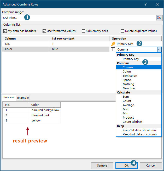
Արդյունք

- Այս հատկությունը կիրառելու համար խնդրում ենք ներբեռնեք և տեղադրեք Kutools Excel-ի համար առաջին.
- Այս հատկության մասին ավելին իմանալու համար դիտեք այս հոդվածը. Արագ համադրեք նույն արժեքները կամ կրկնօրինակեք տողերը Excel-ում
Միացրեք բջիջները, եթե նույն արժեքը VBA կոդի հետ
Դուք կարող եք նաև օգտագործել VBA կոդը՝ սյունակում բջիջները միացնելու համար, եթե նույն արժեքը կա մեկ այլ սյունակում:
1. Մամուլ ալտ + F11 բացել ստեղները Microsoft Visual Basic ծրագրեր պատուհան.
2. Մեջ Microsoft Visual Basic ծրագրեր պատուհանը, սեղմեք Տեղադրել > Մոդուլներ, Ապա պատճենեք և կպցրեք կոդը ներքևում Մոդուլներ պատուհան.
VBA կոդ. Միաձուլված բջիջներ, եթե նույն արժեքները
Sub ConcatenateCellsIfSameValues()
	Dim xCol As New Collection
	Dim xSrc As Variant
	Dim xRes() As Variant
	Dim I As Long
	Dim J As Long
	Dim xRg As Range
	xSrc    = Range("A1", Cells(Rows.Count, "A").End(xlUp)).Resize(, 2)
	Set xRg = Range("D1")
	On Error Resume Next
	For I = 2 To UBound(xSrc)
		xCol.Add xSrc(I, 1), TypeName(xSrc(I, 1)) & CStr(xSrc(I, 1))
	Next I
	On Error GoTo 0
	ReDim xRes(1 To xCol.Count + 1, 1 To 2)
	xRes(1, 1) = "No"
	xRes(1, 2) = "Combined Color"
	For I = 1 To xCol.Count
		xRes(I + 1, 1) = xCol(I)
		For J = 2 To UBound(xSrc)
			If xSrc(J, 1) = xRes(I + 1, 1) Then
				xRes(I + 1, 2) = xRes(I + 1, 2) & ", " & xSrc(J, 2)
			End If
		Next J
		xRes(I + 1, 2) = Mid(xRes(I + 1, 2), 2)
	Next I
	Set xRg = xRg.Resize(UBound(xRes, 1), UBound(xRes, 2))
	xRg.NumberFormat = "@"
	xRg = xRes
	xRg.EntireColumn.AutoFit
End SubNotes:
3. Սեղմեք F5 կոդը գործարկելու բանալին, ապա դուք կստանաք համակցված արդյունքներ նշված տիրույթում:

Excel- ի համար Kutools- ի հետ նույն արժեքը հեշտությամբ միացրեք բջիջներին
Գրասենյակի արտադրողականության լավագույն գործիքները
Լրացրեք ձեր Excel-ի հմտությունները Kutools-ի հետ Excel-ի համար և փորձեք արդյունավետությունը, ինչպես երբեք: Kutools-ը Excel-ի համար առաջարկում է ավելի քան 300 առաջադեմ առանձնահատկություններ՝ արտադրողականությունը բարձրացնելու և ժամանակ խնայելու համար: Սեղմեք այստեղ՝ Ձեզ ամենաշատ անհրաժեշտ հատկանիշը ստանալու համար...
")
Office Tab- ը Tabbed ինտերֆեյսը բերում է Office, և ձեր աշխատանքը շատ ավելի դյուրին դարձրեք
- Միացնել ներդիրներով խմբագրումը և ընթերցումը Word, Excel, PowerPoint- ով, Հրատարակիչ, Access, Visio և Project:
- Բացեք և ստեղծեք բազմաթիվ փաստաթղթեր նույն պատուհանի նոր ներդիրներում, այլ ոչ թե նոր պատուհաններում:
- Բարձրացնում է ձեր արտադրողականությունը 50%-ով և նվազեցնում մկնիկի հարյուրավոր սեղմումները ձեզ համար ամեն օր:
")