Բաց թողնել հիմնական բովանդակությունը

Ինչպե՞ս տեսակավորել այբբենական թվերը Excel- ում:

Եթե ​​ունեք տվյալների ցուցակ, որոնք խառնված են ինչպես թվերի, այնպես էլ տեքստի տողերի հետ, Excel- ում այս սյունակի տվյալները սովորաբար տեսակավորելիս բոլոր մաքուր թվերը դասավորված են վերևում, իսկ ներքևում ՝ խառը տեքստի տողերը: Բայց ձեր անհրաժեշտ արդյունքը, ինչպես ցույց է տրված վերջին սքրինշոթը: Այս հոդվածը կտա օգտակար մեթոդ, որը կարող եք օգտագործել Excel- ում այբբենական թվեր տեսակավորելու համար, որպեսզի կարողանաք հասնել ձեր ուզած արդյունքին:

Տեսակավորեք այբբենական թվերը ՝ բանաձևի օգնականի սյունակով

Բնօրինակ տվյալներ   Սովորաբար տեսակավորեք արդյունքը   ձեր ցանկալի տեսակավորման արդյունքը
Doc տեսակ այբբենական 1 2 Doc տեսակ այբբենական 2 2 Doc տեսակ այբբենական 3

նետ կապույտ աջ պղպջակ Տեսակավորեք այբբենական թվերը ՝ բանաձևի օգնականի սյունակով

Excel- ում դուք կարող եք ստեղծել բանաձևի օգնականի սյուն և այնուհետև տեսակավորել տվյալներն ըստ այս նոր սյունակի, կատարեք հետևյալ քայլերը.

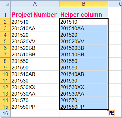
1, Մուտքագրեք այս բանաձևը = TEXT (A2, "###") ձեր տվյալներից բացի, դատարկ բջիջի մեջ, օրինակ, B2, տես նկարի նկարը.

Doc տեսակ այբբենական 4

2, Դրանից հետո քաշեք լրացման բռնակը ներքև դեպի այն բջիջները, որոնք ցանկանում եք կիրառել այս բանաձևը, տես նկարի նկարը.

Doc տեսակ այբբենական 5

3, Եվ ապա տեսակավորեք տվյալները ըստ այս նոր սյունակի, ընտրեք ձեր ստեղծած օգնականի սյունը, ապա կտտացրեք Ամսաթիվ > Տեսակ, և դուրս եկած հուշման վանդակում ընտրեք Ընդլայնել ընտրությունը, տես սքրինշոթեր.

Doc տեսակ այբբենական 6 2 Doc տեսակ այբբենական 7

4, եւ սեղմեք Տեսակ կոճակը բացելու համար Տեսակ երկխոսություն, տակ Սյունակ Բաժին ընտրել Օգնական սյուն անուն, որը ցանկանում եք տեսակավորել և օգտագործել Արժեքներն տակ Տեսակավորել բաժինը, ապա ընտրեք տեսակավորման կարգը, ինչպես ուզում եք, տես նկարի նկարը.

Doc տեսակ այբբենական 8

5. Եվ այնուհետեւ կտտացրեք OK, դուրս եկած Տեսակավորված նախազգուշացման երկխոսությունում ընտրեք Առանձին դասավորեք որպես տեքստ պահված թվերն ու թվերը, տես նկարի նկարը.

Doc տեսակ այբբենական 9

6. Այնուհետեւ կտտացրեք OK կոճակը, կտեսնեք, որ տվյալները տեսակավորված են ըստ ձեր պահանջի:

Doc տեսակ այբբենական 10

7, Վերջապես, ըստ անհրաժեշտության, կարող եք ջնջել օգնող սյունակի պարունակությունը:

Գրասենյակի արտադրողականության լավագույն գործիքները

🤖 Kutools AI օգնականՀեղափոխություն կատարել տվյալների վերլուծության հիման վրա՝ Խելացի կատարում   |  Ստեղծեք ծածկագիր  |  Ստեղծեք հատուկ բանաձևեր  |  Վերլուծել տվյալները և ստեղծել գծապատկերներ  |  Invoke Kutools-ի գործառույթները...
Հանրաճանաչ հատկություններ: Գտեք, ընդգծեք կամ նույնականացրեք կրկնօրինակները   |  Deleteնջել դատարկ շարքերը   |  Միավորել սյունակները կամ բջիջները՝ առանց տվյալների կորստի   |   Կլոր առանց բանաձևի ...
Super Փնտրել: Բազմաթիվ չափանիշների VLookup    Բազմակի արժեք VLookup  |   VLookup բազմաթիվ թերթերում   |   Fuzzy Փնտրել ....
Ընդլայնված բացվող ցուցակ: Արագ ստեղծեք բացվող ցուցակը   |  Կախված բացվող ցուցակ   |  Բազմակի ընտրություն Drop Down ցուցակ ....
Սյունակի կառավարիչ: Ավելացրեք որոշակի քանակությամբ սյունակներ  |  Տեղափոխել սյունակները  |  Փոխարկել թաքնված սյունակների տեսանելիության կարգավիճակը  |  Համեմատեք միջակայքերը և սյունակները ...
Առանձնահատկություններ: Ցանցի կենտրոնացում   |  Դիզայնի տեսք   |   Մեծ Formula Bar    Աշխատանքային գրքույկի և թերթիկների կառավարիչ   |  Ռեսուրսների գրադարան (Ավտոմատ տեքստ)   |  Ամսաթիվ ընտրող   |  Միավորել աշխատանքային թերթերը   |  Գաղտնագրել/գաղտնազերծել բջիջները    Ուղարկեք նամակներ ըստ ցանկի   |  Սուպեր զտիչ   |   Հատուկ զտիչ (զտել թավ/շեղ/շեղված...) ...
Լավագույն 15 գործիքների հավաքածու12 Տեքստ Գործիքներ (Ավելացրեք տեքստ, Հեռացնել նիշերը, ...)   |   50+ Աղյուսակ Տեսակներ (Գանտի աղյուսակը, ...)   |   40+ Գործնական Բանաձեւեր (Հաշվարկել տարիքը ՝ ելնելով ծննդյան տարեդարձից, ...)   |   19 միացում Գործիքներ (Տեղադրեք QR կոդ, Տեղադրեք նկար ուղուց, ...)   |   12 Փոխարկում Գործիքներ (Բառեր համարներ, Արտարժույթի փոխակերպումը, ...)   |   7 Միաձուլում և պառակտում Գործիքներ (Ընդլայնված կոմբինատ տողեր, Պառակտված բջիջներ, ...)   |   ... եւ ավելին

Լրացրեք ձեր Excel-ի հմտությունները Kutools-ի հետ Excel-ի համար և փորձեք արդյունավետությունը, ինչպես երբեք: Kutools-ը Excel-ի համար առաջարկում է ավելի քան 300 առաջադեմ առանձնահատկություններ՝ արտադրողականությունը բարձրացնելու և ժամանակ խնայելու համար:  Սեղմեք այստեղ՝ Ձեզ ամենաշատ անհրաժեշտ հատկանիշը ստանալու համար...

Նկարագրություն


Office Tab- ը Tabbed ինտերֆեյսը բերում է Office, և ձեր աշխատանքը շատ ավելի դյուրին դարձրեք

  • Միացնել ներդիրներով խմբագրումը և ընթերցումը Word, Excel, PowerPoint- ով, Հրատարակիչ, Access, Visio և Project:
  • Բացեք և ստեղծեք բազմաթիվ փաստաթղթեր նույն պատուհանի նոր ներդիրներում, այլ ոչ թե նոր պատուհաններում:
  • Բարձրացնում է ձեր արտադրողականությունը 50%-ով և նվազեցնում մկնիկի հարյուրավոր սեղմումները ձեզ համար ամեն օր:
Comments (10)
No ratings yet. Be the first to rate!
This comment was minimized by the moderator on the site
The stock symbol for TrueCar Inc is "TRUE". When I sort the column containing the stock symbols, TRUE falls out of place at the end of the list. The cell is formatted as text. I am assuming that it is because "TRUE" has special meaning in Excel. Right now I am removing the "E", sorting the column so the row falls in the right place and then adding the E after the sort. Any ideas on a better approach?  
This comment was minimized by the moderator on the site
Hi, I have a similar sorting requirement, but with a unique problem ....
I have a range of Stock data which I need to sort in Category order.
The Range includes prices and one column has formulas.
The Category numbers range from 1 1a 1b etc to 32e.
I have continuously tried using a helper column with the formula =TEXT(K3,"###") - with K3 being the first Row in the Category column.
I select the helper column (N) and click Data - Sort - Expand the selection, but get no further as the "expansion" always selects from Row 40 - even if I select just a few rows in the helper column.
Why is this, and how can I sort my data correctly ?
Looking forward to a solution ....
Thanks.
Patrick.
This comment was minimized by the moderator on the site
Thanks for the tip on using a "helper column", but here's my question:

Is there a way to get the "related " columns to "tag along" with the sort precipitated by the helper column?

For example, column A contains a mixed-string product code that I can now sort into sequence using the "helper column" technique but, attached to that same product code are product descriptions, dimensions and other characteristics (some of which are also mixed-string in nature) in several other columns, and I need those to follow the "helper column" sort.

Any suggestions?

Much appreciated!

Lorne
This comment was minimized by the moderator on the site
I only see 1 method. Top of the article mentions that we will see 2 methods.
This comment was minimized by the moderator on the site
Hello, val,
Thank you for your comment, it is my mistake, I have deleted the second method from this article, and now, I have updated the article.

Thank you once more!
This comment was minimized by the moderator on the site
Trying to sort Alphanumeric with text. It is a fairly large list but below is an example. I can't strip the off the letter in a different column and sort by that because I have matching numbers that should come before them. I also can't really add a column to sort by and then hide that column - or delete it because I am constantly sorting the data. Any ideas? Will there be some formula? My current list: ---- What I want it to look like: 1 ---- 1 2 ---- 2 3 ---- 3 4 ---- 4 A1 ---- A1 A10 ---- A2 A100 ---- A3 A2 ---- A4 A20 ---- A5 A200 ---- A6 A3 ---- A7 A4 ---- A8 A5 ---- A9 A6 ---- A10 A60 ---- A20 A7 ---- A60 A8 ---- A100 A9 ---- A200
This comment was minimized by the moderator on the site
The easiest way I can think is to split the column into the Alpha part ("A") and the numeric part ("1") and then sort first by alpha then by numeric.
Your original 1,2,3,4 would need to stay in the alpha column to sort properly .

N.B. this might be a bit more difficult to achieve when the alpha part (the "A") is not a consistent length in your data. But definitely still possible.
This comment was minimized by the moderator on the site
I am running in the same problem. I have 1200 part numbers that I need to sort the way it's shown above but excel will put V15 after V1 if V14 is absent. I need V14 to appear after V9 or V8, where ever the part number ends.
This comment was minimized by the moderator on the site
Trying to sort Alphanumeric with text. It is a fairly large list but below is an example. I can't strip the off the letter in a different column and sort by that because I have matching numbers that should come before them. I also can't really add a column to sort by and then hide that column - or delete it because I am constantly sorting the data. Any ideas? My current list: ---- What I want it to look like: 1 ---- 1 2 ---- 2 3 ---- 3 4 ---- 4 A1 ---- A1 A10 ---- A2 A100 ---- A3 A2 ---- A4 A20 ---- A5 A200 ---- A6 A3 ---- A7 A4 ---- A8 A5 ---- A9 A6 ---- A10 A60 ---- A20 A7 ---- A60 A8 ---- A100 A9 ---- A200
This comment was minimized by the moderator on the site
When I do this, the column sorts by individual character and I don't get the right order. For instance, if I have the following data: A1: 1 A2: 2 A3: 1a1 A4: 12 A5: 1a2 I want them to be sorted like this: A1: 1 A2: 1a1 A3: 1a2 A4: 2 A5: 12 Just sorting the column normally I end up with this: A1: 1 A2: 2 A3: 12 A4: 1a1 A5: 1a2 Where the numbers are sorted correctly and then the alphanumeric values are sorted correctly, but the two are not sorted together. When I use the method in the article, I end up with this: A1: 1 A2: 12 A3: 1a1 A4: 1a2 A5: 2 Where the numeric and alphanumeric data are sorted together but incorrectly (12 should come after 2). Why is this happening?
There are no comments posted here yet
Please leave your comments in English
Posting as Guest
×
Rate this post:
0   Characters
Suggested Locations